Primality Testing and Factoring
In this handout we consider the problems of testing numbers for primality and factoring integers into primes. We've seen these problems come up many times in this course. For example, generating RSA keys requires primality testing and RSA can be broken by factoring integers. This state of affairs is possible because algorithms for primality testing are very fast, while algorithms for factoring integers (at least the currently known ones) are very slow.
In this worksheet we will assume that $p$ is odd (since when $p$ is even primality testing is trival).
Fermat's little theorem
Much of this handout is based on extensions of Fermat's little theorem. Recall that this says that if $p$ is prime and $a$ is coprime to $p$ (i.e., $\renewcommand{\Z}{\mathbb{Z}}a\in\Z^*_p$) then
\begin{align*} a^{p-1} &\equiv 1 \pmod{p} . \end{align*}
Also recall that we used the existence of primitive roots in $\Z^*_p$ in the Diffie–Hellman protocol. In other words, there is a primitive root $\omega\in\Z^*_p$ that generates every element by taking powers of it; i.e, $\Z^*_p=\{1,2,\dotsc,p-1\}=\{\omega,\omega^2,\dotsc,\omega^{p-1}\}$. This means that $\Z^*_p$ is a cyclic group under multiplication.
One important consequence of this is that there are exactly two solutions to the equation $x^2=1$ in $\Z^*_p$. It is easy to see what these solutions are, since both $x=1$ and $x=-1$ when squared give $1$. We have $\omega^{p-1}=1$ by Fermat's little theorem and the other solution must be $\omega^{(p-1)/2}=-1$ since $\Z^*_p$ is cyclic.
In other words, the only square roots of $1$ in $\Z^*_p$ are $\pm1$. Note that this is not true when $p$ is not prime, e.g., $3^2=1$ in $\Z^*_8$ and yet $3\neq\pm1$ in $\Z^*_8$.
The square root of Fermat's little theorem
Let $x=a^{(p-1)/2}$ ($p$ is odd, so the exponent is an integer) and Fermat's little theorem implies $x^2=1$ in $\Z^*_p$. Since this implies $x=\pm1$ we have that
\begin{align*} a^{(p-1)/2} &\equiv \pm 1 \pmod{p} \qquad\text{for all $a\in\Z^*_p$} \end{align*}
which can intuitively be considered the "square root" of Fermat's little theorem.
The fourth root
Furthermore, consider the case when $a^{(p-1)/2}\equiv 1\pmod{p}$ and $(p-1)/2$ is even. In such a case a similar argumentation as above (but setting $x=a^{(p-1)/4}$) gives $a^{(p-1)/4}\equiv\pm1\pmod{p}$.
Generalization
We can generalize this "square-rooting" process as follows.
Write $p-1$ in the form $2^s\cdot t$ where $s$ is a positive integer and $t$ is odd. Since $p-1$ is even and has a unique prime factorization this can always be done in a unique way.
If $p=2^s\cdot t+1$ is prime and $a\in\Z^*_p$ then the sequence
\begin{equation*} (a^{2^s\cdot t}, a^{2^{s-1}\cdot t}, a^{2^{s-2}\cdot t}, \dotsc, a^{t}) \end{equation*}
of numbers in $\Z^*_p$ must have the form
\begin{equation*} (1,1,\dotsc,1,-1,*,*,\dotsc,*) \qquad\text{where ‘$*$’ is arbitrary and not $\pm1$} \end{equation*}
or the sequence could consist of all 1s (if $a^{(p-1)/n}$ for $n=2,4,\dotsc,2^s$ is always $1$ and never $-1$).
This observation is very useful for primality testing.
Stronger primality testing
We've seen that Fermat's little theorem provides a simple primality test (or more technically a compositeness test since it actially detect composites, not primes). To perform the test, take a random $a\in\Z^*_p$ and compute $a^{p-1}\in\Z^*_p$. If $a^{p-1}\neq 1$ then $p$ is composite. If $a^{p-1}=1$ then we can't say anything (but maybe we have a suspicion that $p$ is prime). However, we can select another $a\in\Z^*_p$ and try the test again.
Although this test is very elegant, there are some composite numbers $p$ that always "look prime", regardless of what value of $a$ is selected. Such numbers are called Carmichael numbers after Robert Carmichael who in 1910 discovered the smallest such number, 561:
# Compute the a for which a^561 != a modulo 561
l = [a for a in (0..560) if power_mod(a, 561, 561) != a]
print("The a for which a^561 - a is not divisible by 561:", l)
print("Yet 561 = {} is not prime".format(factor(561)))
Actually, the Czech mathematician Václav Šimerka found the first 7 Charmichael numbers 25 years before Carmichael but his paper was written in Czech and unfortunately not noticed, at least in the English-speaking world.
In 1994, Alford, Granville, and Pomerance showed that there are infinitely many Charmichael numbers. Although they are relatively rare it makes the Fermat test less than desirable knowing that there are infinitely many composite numbers that it cannot detect.
However, the generalization of Fermat's little theorem we derived above fairs much better. The idea is to compute the sequence
\begin{equation*} (a^{2^s\cdot t}, a^{2^{s-1}\cdot t}, a^{2^{s-2}\cdot t}, \dotsc, a^{t}) \in (\Z^*_p)^{s+1} \end{equation*}
from above and check that it is of the form
\begin{equation*} (1,1,\dotsc,1,-1,*,*,\dotsc,*) \qquad\text{or}\qquad (1,1,\dots,1) . \end{equation*}
The easiest way to do this is start from the right-hand side and look for a $-1$ appearing in the sequence. As soon as either a $1$ or $-1$ is reached all entries to its left must be $1$ (since $\pm1$ squared is $1$) and therefore we only have to compute the sequence until a $\pm1$ is reached.
Computing each entry from scratch would be wasteful; the $k$th entry is the square of the $(k+1)$th entry, so moving one entry to the left just requires a single squaring. Also, if we have reached the second entry in the vector and have still not seen $\pm1$ we know the sequence cannot be of the required form (as if $p$ is prime then the very first entry is always $1$ by Fermat, meaning the second entry must be $\pm1$).
Strong primality test pseudocode
Given odd $p$, find $s$ and $t$ such that $p-1=2^s\cdot t$.
Choose $a\in\Z^*_p$ randomly.
Set $b:=a^t\bmod p$.
If $b\equiv\pm1\pmod{p}$ then return probably prime.
Repeat $s-1$ times:
$\hspace{1em}$ $b:=b^2\bmod p$
$\hspace{1em}$ If $b\equiv-1\pmod{p}$ then return probably prime.
$\hspace{1em}$ If $b\equiv1\pmod{p}$ then return composite.
Return composite.
Analysis
Computing $b$ initially uses $\renewcommand{\M}{\mathop{\mathsf{M}}}O(\log t\M(\log p))$ word operations via repeated squaring, where $\M(b)$ is the multiplication cost of two $b$-bit numbers. Each loop iteration uses a single squaring (mod $p$) and there are at most $s-1$ loop iterations for a total cost of $O(s\M(\log p))$ word operations.
Since $t=O(p)$ and $s=O(\log p)$ the total cost is $O(\log p\M(\log p))$.
Effectiveness
One can prove that if $p$ is an odd composite then the number of $a\in\Z^*_p$ for which this algorithm will return "probably prime" is at most $|\Z^*_p|/4$. In other words, there is at most a 25% chance that the algorithm will incorrectly think a composite is prime.
However, there are no more Carmichael numbers to worry about: regardless of the input at least 75% of the choices for $a$ will produce a correct answer.
Miller–Rabin test
What makes the strong primality test even more effective is that there is nothing stopping you from applying it multiple times. If the algorithm returns "composite" then you can immediately stop, but if the algorithm returns "probably prime" then you can run the algorithm repeatedly, each time choosing a different random choice for $a$. If the random choices are independent this provides a very effective test.
Say the algorithm returns "probably prime" 100 times in a row. What is the chance that $p$ is actually composite and the test failed every time? The probability that it fails 100 times in a row is at most $(1/4)^{100}$ which is too small to reason about. You're more likely to win the Lotto 6/49 eight times in a row. On the other hand, this is only an "experimental" proof, not a mathematical one.
Running the strong primality test multiple times to randomly choosen bases is known as the Miller–Rabin test. By iterating the test enough times you can easily make the probability of failure as small as you like and it practice this is good enough. Even better, the $1/4$ error rate is vastly too pessimistic in practice and for large $p$ even a single "probably prime" makes it quite likely that $p$ is in fact prime. It has been shown by Damgård, Landrock, and Pomerance that a random $k$-bit number will be mischaracterized by the strong primality test with probability at most $k^2\cdot4^{2-\sqrt{k}}$ and this approaches 0 as $k\to\infty$.
Primality proving
What if you are not satisfied with an arbitrarily small (even minuscule) possibility of error and you want a mathematical proof that a number $p$ is prime? Again, an extension of Fermat's little theorem can be used.
The order of an element $a\in\Z^*_p$ is the smallest positive power $k$ that gives $a^k=1$ in $\Z^*_p$. We've seen that primitive roots exist in $\Z^*_p$. By definition, this means that there is an $\omega\in\Z^*_p$ such powers of $\omega$ generate all of $\Z^*_p$, i.e., $\{\omega,\omega^2,\dotsc,\omega^{p-1}\}=\Z^*_p$. In other words, the order of a primitive root $\omega$ is $p-1$ exactly.
This property can be used to prove primality, since if $n$ is not prime then we know that not every element of $\{1,2,\dotsc,n-1\}$ is invertible. For example, if $p$ is a prime divisor of $n$ then $p$ itself is not invertible, since $\gcd(n,p)>1$.
In summary, $\Z^*_n$ denotes the group of residues mod $n$ that are invertible and $\phi(n)$ denotes the size of this group. When $n$ is prime, $\phi(n)=n-1$ because all nonzero residues are invertible. When $n$ is composite, $\phi(n) < n-1$ because some nonzero residues are not invertible. However, there is no known way of computing $\phi(n)$ efficiently unless the factorization of $n$ is known.
Finding an element of large order
In order to prove $p$ is prime we will find an element of $\Z^*_p$ of the largest possible order $p-1$. This demonstrates that $p$ must be prime, otherwise an element of such a large order could not exist.
Even if we find an element $a$ of order $p-1$, how can we efficiently compute its order? Computing $a$, $a^2$, $a^3$, $\dots$, $a^{p-2}$ and verifying they are all nonzero would be very slow, requiring $p-3$ multiplications by $a$. This is exponential in $\log p$.
There is a better way of computing the order of an element, but there is a catch—it requires knowing all the prime factors of $p-1$. But if we can find these somehow the following fact can be used:
Suppose $q_1$, $\dotsc$, $q_l$ are all prime factors of $p-1$. Then $a$ has order $p-1$ if:
\begin{align*} a^{p-1} &\equiv 1\pmod{p} \\ a^{(p-1)/q_i} &\not\equiv 1\pmod{p} \text{ for all $1\leq i\leq l$}. \end{align*}
Proof
Suppose $a$ satisfies the given congruences. In order to reach a contradiction, suppose there is some $u<p-1$ for which $a^u\equiv 1\pmod{p}$. Now consider $\gcd(u,p-1)=g$. By the Euclidean algorithm (Bézout's identity) we can write $g=su+t(p-1)$ for some $s,t\in\Z$. Then
\begin{equation*} a^g \equiv a^{su+t(p-1)} \equiv (a^u)^s\cdot(a^{p-1})^t \equiv 1^s\cdot1^t \equiv 1\pmod{p} . \tag{$*$} \end{equation*}
Since $g$ divides $p-1$ we must have $g=(p-1)/Q$ where $Q$ is a product of the prime divisors of $p-1$. Also, $g$ divides $u<p-1$ so we must have $g<p-1$ which implies $Q>1$.
Suppose $q_i$ is one of the prime divisors of $Q$. Then raising ($*$) by $Q/q_i$ gives
\begin{equation*} a^{gQ/q_i} \equiv a^{(p-1)/q_i} \equiv 1 \pmod{p} \end{equation*}
which contradicts the given congruence $a^{(p-1)/q_i} \not\equiv 1 \pmod{p}$. Thus there must be no $u<p-1$ for which $a^u\equiv1\pmod{p}$, i.e., $a$ is of order $p-1$.
Example
The $p-1$ test works best when $p-1$ factorizes nicely. For example, it can easily be used to show that $p=3\cdot2^{353}+1$ is prime. Note that the only prime factors of $p-1$ are $2$ and $3$.
p = 3*2^353 + 1
a = 5
print(power_mod(a, p-1, p) == 1)
print(power_mod(a, Integer((p-1)/2), p) != 1)
print(power_mod(a, Integer((p-1)/3), p) != 1)
Since $5^{p-1}\equiv1\pmod{p}$ but $5^{(p-1)/2}\not\equiv1\pmod{p}$ and $5^{(p-1)/3}\not\equiv1\pmod{p}$ it follows by the $p-1$ test that $5$ has order $p-1$ in $\Z^*_p$ and therefore $p$ is prime.
Caveat 1
If the prime factorization of $p-1$ is unknown then the test cannot be used. Unfortunately, $p-1$ is approximately the same size as $p$ and factorizing a number is much more difficult than testing its primality. Unless you get lucky there is no reason to expect that the prime factorization of $p-1$ can be efficiently computed for general numbers $p$.
However, sometimes you don't have a specific prime in mind and just want to prove some number is prime. For example, finding a prime to use in the Diffie–Hellman protocol. In such a case the prime can be chosen to be of the form $\prod_i q_i^{e_i}+1$ for known primes $q_i$ and some choice of exponents $e_i$. Once a choice is found that produces a prime number that number can easily be proven prime using the $p-1$ test (and as a side effect produces a primitive root $a\in\Z^*_p$ which is also required for Diffie–Hellman). For Diffie–Hellman security, at least one prime factor $q_i$ of $p-1$ should be large.
Caveat 2
Assuming the factorization of $p-1$ is known then what method can we use to select a primitive root $a\in\Z^*_p$? If we want a deterministic (non-random) algorithm there is no efficient algorithm that can be proven to work in all cases.
However, in practice this problem is not difficult using randomness: simply try random $a\in\Z^*_p$ until one works! This might seem inefficient, but in fact many elements of $\Z^*_p$ are primitive elements. To be precise, there are $\phi(p-1)$ primitive elements in $\Z^*_p$ and this grows like $\Theta(p/\log\log p)$. In other words, in practice a random $a\in\Z^*_p$ has about a $1/\log\log p$ chance of being primitive. Thus finding a primitive element will usually take about $\log\log p$ selections for $a$ since you are unlikely to be repeatedly unlucky over and over again.
The $p+1$ test
As an aside, sometimes there are cases where the prime factorization of $p-1$ cannot be found but the prime factorization of $p+1$ is known. In such cases, a variant of the $p-1$ test can be used which replaces $p-1$ with $p+1$. The primary difference is that the $p+1$ test performs operations in $\mathbb{F}^*_{p^2}$ instead of $\mathbb{F}^*_p$. For this reason the arithmetic done in the $p+1$ test is approximately twice as slow meaning that the $p-1$ test is preferable if possible.
Factoring
We now turn our attention to the problem of decomposing a number into its prime factorization. In fact, given a number $n$ it is sufficient to find a nontrivial divisor $d$, i.e., a number for which $\gcd(d,n)\not\in\{1,n\}$. Because finding a nontrivial divisor allows splitting the number $n$ as $d\cdot(n/d)$ and the algorithm can be recursively applied to the factors $d$ and $n/d$ until the numbers that remain are primes, in which case the prime factorization of $n$ has been computed.
Trial division
The most straightforward way of finding nontrivial factors is to test $n$ for divisibility by the primes $2$, $3$, $5$, $7$, $11$, $\dotsc$ in order. When can you stop? If $n$ is not prime then it must have a nontrivial divisor less than or equal to $\sqrt{n}$, so we only need to check for divisibility by primes $p\leq\sqrt{n}$.
The prime number theorem
How many primes are there up to $\sqrt{n}$? The notation $\pi(x)$ is used to count how many primes there are $\leq x$, so there are $\pi(\sqrt{n})$ primes up to $\sqrt{n}$.
The prime number theorem says that $\lim_{x\to\infty}\frac{\pi(x)}{x/\ln x} = 1$. In other words, $\pi(x)\approx x/\ln x$ as $x$ gets large. A weaker form of this which is sufficient for our analysis is that $\pi(x)=\Theta(x/\log x)$.
Analysis
First, suppose we have a list of all primes $p_1,\dotsc,p_k\leq\sqrt{n}$ where $k=\pi(\sqrt{n})=O(\sqrt{n}/\log n)$.
Trial division requires $k$ divisions of numbers with $\log n$ words. Total cost is $O(k(\log n)^2)=O(\sqrt{n}\log n)$ word operations. This is exponential in $\log n$ and so trial division will run slowly even if the list of primes is known in advance.
Generating a list of primes
How could the list of primes be computed, though? The sieve of Eratosthenes (an algorithm that dates back to the third century BC) provides a way of doing this which is much better than using a primality test on each prime candidate individually.
In order to determine all the primes up to $n$ first initialize a Boolean array $A$ of length $n-1$ (indexed from $2$ to $n$) to contain $1$s, i.e., $A[2]=1$, $\dotsc$, $A[n]=1$.
Now set even-index entries of $A$ (except for $A[2]$) to 0, i.e., $A[4]=0$, $A[6]=0$, $\dotsc$, since $4$, $6$, $\dotsc$, are all even composites.
Now set $A[i]=0$ where $i=3k$ for $k>1$ (this removes all composite multiples of three).
Then $A[i]=0$ where $i=5k$ for $k>1$ (removing all multiples of 5), etc.
Continue in this process until the multiples of all primes $p\leq\sqrt{n}$ have been removed. The remaining indices $p$ for which $A[p]=1$ are exactly the primes $p\in[2,n]$.
There are $O(n\log\log n)$ array elements set to 0 during this process; computing the indices to operate on uses addition on integers up to $n$ (adding an extra $\log n$ cost). This algorithm also uses $O(n)$ space which limits it to being used to generate relatively short lists of primes.
The $p-1$ factoring method
Fermat's little theorem also form the basis of a factoring method developed by John Pollard in 1974. The idea is that if $p$ is a prime divisor of $n$ and $M$ is a multiple of $p-1$ then $a^M\equiv1\pmod{p}$ or equivalently $p$ divides $a^M-1$. It follows that $\gcd(a^M-1,n)\geq p$.
Thus, a nontrivial factor of $n$ can be recovered by computing the greatest common divisor of $a^M-1\bmod n$ and $n$ (except when this GCD happens to be $n$ itself).
What's the issue here? Well, $M$ was selected to be a multiple of $p-1$. But we don't know what $p$ is; as a prime divisor of $n$ it is what we are trying to find in the first place.
However, sometimes it happens that $p-1$ is a "smooth" number meaning that its prime factorization consists of lots of small prime factors and no large prime factors. In such a case it is not too difficult to compute a multiple of $p-1$ by just multiplying a lot of small primes together.
For example, define $M(x)$ as the least common multiple of $\{2,3,\dotsc,x\}$. This number consists of the product of a lot of small primes and can easily be computed by generating all primes up to $x$ via the sieve of Eratosthenes. To compute $M(x)$ you also need to compute all the prime powers up to $x$ but that is easy to do once the primes are known.
For example, to compute $M(10)$ we first find the primes up to 10: 2, 3, 5, 7. By taking powers of 2, we find that $2^3$ is the largest power of 2 less than 10 and similarly that $3^2$ is the largest power of 3 less than 10. Since $5^2>10$ and $7^2>10$ it follows that $M(10)=2^3\cdot3^2\cdot5\cdot7$.
Once $M(B)$ has been computed for some bound $B$ we can attempt to factor $n$ by selecting an $a\in\Z^*_n$ and computing $a^{M(B)}-1$ in $\Z^*_n$ by using repeated squaring modulo $n$. Finally, we can use Euclid's algorithm to compute $\gcd(a^{M(B)}-1,n)$ and see if this is nontrivial.
Typical case
Unfortunately, typically what happens is that $\gcd(a^{M(B)}-1,n)=1$ which indicates that $n$ has no prime factors $p$ such that $M(B)$ is a multiple of $p-1$. In such a case $B$ could be increased and the method tried again, but often $n$ will have no prime divisors for which $p-1$ is particularly smooth meaning that $B$ would have to be taken far too large for the method to be feasible.
Alternative failure case
Another way in which the method could fail is if $\gcd(a^{M(B)}-1,n)=n$. In such a case increasing $B$ is of no use but computing GCDs more frequently (instead of once at the end) can help.
For example, say $M(B):=\prod_{i=1}^k p_i^{e_i}$ where $p_i$ is the $i$th prime. Then one could could compute $a^{M(B)}\bmod n$ via the pseudocode:
$b:=a$
for $i$ from $1$ to $k$:
$\hspace{1em}$ repeat $e_i$ times:
$\hspace{2em}$ $b := b^{p_i}\bmod n$
Immediately after each exponentiation one can check if $\gcd(b-1,n)$ is nontrivial.
Sometimes even this is not enough because all $p-1$ (for $p$ dividing $n$) might have the same largest prime divisor. There is a workaround for this: do the outer loop backwards so that the squarings come last. If $a$ is chosen randomly and $n$ has at least 2 odd prime factors one can show that at least 50% of the time $\gcd(b-1,n)$ will be nontrivial after some squaring. Essentially this is because if $p$ and $q$ are two odd prime divisors of $n$ then if you find an $a$ satisfying
\begin{equation*} a^{M(B)/2^i}\equiv 1\pmod{p} \qquad\text{and}\qquad a^{M(B)/2^i}\equiv -1\pmod{q} \qquad\text{(for some $i$)} \end{equation*}
then $p$ will divide $a^{M(B)/2^i}-1$ but $q$ will not, so $\gcd(a^{M(B)/2^i}-1,n)\not\in\{1,n\}$.
Analysis
All the arithmetic is performed modulo $n$ which is polynomial time in $\log n$. Computing $a^{M(B)}$ takes $O(\log(M(B))(\log n)^2)$ operations using schoolbook multiplication, for example. The prime number theorem can be used to show this is $O(B(\log n)^2)$ which is exponential in $\log B$.
Pollard's rho method
The Pollard "$\rho$" method, named because it uses a specific periodic sequence of numbers which when written out is shaped like a $\rho$. Given a number $n$ to factor, the idea is to use a function $f\colon\Z_n\to\Z_n$ and a starting seed $s$ and compute the sequence of numbers
\begin{equation*} s, f(s), f(f(s)), f(f(f(s))), \dotsc . \end{equation*}
Because $\Z_n$ is finite this sequence is necessarily periodic; as soon as two distinct $i,j$ are found with $f^i(s)=f^j(s)$ it follows that $f^{i+1}(s)=f^{j+1}(s)$, etc. There may also be a "preperiod" before the periodic portion starts but once the periodic part starts it will never stop. This is where the name comes from: the periodic part forms the oval of the $\rho$ and there may be a nonperiodic part which forms the tail of the $\rho$.
For example, the following diagram demonstrates what happens when $n=527$, $s=17$, and $f(x):=x^2+1$.
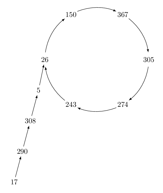
This particular example has a preperiod of $[17,290,308,5]$ (length 4) and a period of $[26,150,367,305,274,243]$ (length 6).
# Applying the iteration f(x) = x^2 + 1 mod 527 starting from 17
n = 527
R.<x> = Zmod(n)[]
f = x^2 + 1
a = [17]
for i in range(16):
    a.append(f(a[-1]))
print(a)
How is this useful for factoring?
Suppose $p$ and $q$ are prime divisors of $n$. Pollard's insight is that the iteration $x\mapsto f(x)$ when applied mod $p$ or $q$ will also produce a periodic sequence. Also, it is often the case that the period of the iteration mod $p$ and the period of the iteration mod $q$ don't match exactly. Of course, since we don't know $p$ and $q$ we can't compute the iterations modulo $p$ and $q$ directly.
But suppose $i$ and $j$ are two indices of the iteration corresponding to the same entry in the cycle mod $p$ but not the same entry in the cycle mod $q$, i.e.,
\begin{equation*} f^i(s) \equiv f^j(s) \pmod{p} \qquad\text{and}\qquad f^i(s)\not\equiv f^j(s) \pmod{q} . \end{equation*}
Then $p$ will divide $f^i(s)-f^j(s)$ but $q$ will not, so $\gcd(f^i(s)-f^j(s), n)$ will be a nontrivial factor of $n$.
In the example above, consider the iteration mod $p=17$ and $q=31$:
print(list(map(lambda x: x % 17, a)))
print(list(map(lambda x: x % 31, a)))
Both have a preperiod of 4, but $f^i(s)\bmod p$ has a period of 6 while $f^i(s)\bmod q$ has a period of 1 (i.e., $f^i(s)\equiv f^j(s)\pmod{q}$ for $i=4$, $j=5$).
Indeed, we have $\gcd(f^5(s)-f^4(s),n)=q$ is a nontrivial factor.
gcd(a[5]-a[4],n)
How to find a cycle?
One important missing part: how can we detect the presence of a cycle, i.e., find $i$ and $j$ such that $f^i(s)=f^j(s)$? Computing $f^i(s)$ for $i=1,2,\dotsc$ is not a problem, but how do we know once we've hit a repeat? One way would be to record the values of $f^i(s)$ that we've seen so that we know when a cycle has occured. However, this requires a method of storing the values, which isn't ideal (and also we don't know the values mod $p$ or $q$). Alternatively, we could exhaustively check for the presence of a cycle by checking if $f^i(s)=f^j(s)$ for all pairs $(i,j)$ up to some large number of steps. This doesn't use any extra space, but is not efficient since there will be a check for each pair $(i,j)$ which grows quadratically in the number of steps.
Floyd's cycle finding algorithm
Amazingly, there is a simple method that can be used to detect a cycle in a periodic sequence that requires only storing two values of the sequence at a time. The idea is to keep track of two pointers while iterating through the sequence, a tortoise pointer that moves one step at a time and a hare pointer that moves twice as fast. Eventually the tortoise and hare must meet and when they do they must be in the periodic part of the sequence.
For example, in the following the green number denotes the tortoise and the red number denotes the hare. After six steps it is determined that 150 is in the periodic part of the sequence.
\begin{gather*} {[{\color{green}{17}},{\color{red}{290}},308,5,26,150,367,305,274,243,26,150,367,305,274,243,26]} \\ {[17,{\color{green}{290}},308,{\color{red}{5}},26,150,367,305,274,243,26,150,367,305,274,243,26]} \\ {[17,290,{\color{green}{308}},5,26,{\color{red}{150}},367,305,274,243,26,150,367,305,274,243,26]} \\ {[17,290,308,{\color{green}{5}},26,150,367,{\color{red}{305}},274,243,26,150,367,305,274,243,26]} \\ {[17,290,308,5,{\color{green}{26}},150,367,305,274,{\color{red}{243}},26,150,367,305,274,243,26]} \\ {[17,290,308,5,26,{\bf\color{green}{150}},367,305,274,243,26,{\bf\color{red}{150}},367,305,274,243,26]} \end{gather*}
Thus, Pollard's $\rho$ method after $i$ steps will keep track of $f^{i}(s)$ and $f^{2i}(s)$. To check if the periodic part of the sequence (mod $p$) is reached the algorithm will compute $\gcd(f^{2i}(s)-f^{i}(s),n)$ and see if this provides a nontrivial factor.
If the GCD is $1$ this indicates the periodic part of the sequence hasn't been reached yet (modulo any prime factor of $n$). Conversely, if the GCD is $n$ itself this indicates the periodic part of the sequence was reached modulo all prime factors of $n$. In such a case the method fails, but we can try another starting seed $s$ or another $f$ such as $f(x):=x^2+a$ for another value of $a$.
Example
Suppose $n=527$, $s=17$, and $f\colon\Z_n\to\Z_n$ defined by $f(x)=x^2+1$.
Step 1: $\gcd(f^2(s)-f^1(s),n)=\gcd(18,527)=1$
Step 2: $\gcd(f^4(s)-f^2(s),n)=\gcd(245,527)=1$
Step 3: $\gcd(f^6(s)-f^3(s),n)=\gcd(362,527)=1$
Step 4: $\gcd(f^8(s)-f^4(s),n)=\gcd(248,527)=31$ is a nontrivial factor of $n$
Optimization
Since computing a GCD is a relatively expensive operation it can pay off to not compute a GCD after every step. Instead of taking a GCD, one can multiply together $f^{2i}(s)-f^{i}(s)\bmod n$ for multiple values of $i$ together and then take a GCD on the entire product. For example, whenever the step counter $i$ is a multiple of 100 you could compute
\begin{equation*} \gcd\Bigl(\prod_{j=i-100}^i (f^{2j}(s)-f^{j}(s)) \bmod n, n\Bigr) . \end{equation*}
This greatly reduces the number of GCDs that have to be performed, though it does have the downside that one is more likely to get the trivial GCD of $n$ using this approach.
However, this downside is easily remedied by saving the values of $f^{i-100}(s)$ and $f^{2(i-100)}(s)$. If the GCD ever becomes $n$ then one can restart the process from the $(i-100)$th step, but this time computing the GCD after every step in case there was a nontrivial GCD that was skipped.
Analysis
For simplicity, suppose that the iterations of the function $f$ produce uniformly random values in $\Z_n$ and $p$ is the smallest prime factor of $n$. Then by the "birthday paradox" with probability $1/2$ there will be a repetition modulo $p$ after $O(\sqrt{p})$ iterations. It is unlikely that the first repetition modulo $p$ and the first repetition modulo $(n/p)$ will occur on exactly the same step, so with probability $1/2$ we expect the Pollard $\rho$ method to find the factor $p$ of $n$ using $O(\sqrt{p}\cdot(\log n)^2)=O(e^{(\log p)/2}(\log n)^2)$ word operations. This is exponential in $\log p$ but it is much better than trial division which needs $\pi(p)\approx p/\log p$ arithmetic operations in order to find $p$.
Fermat's method
In 1643, the French lawyer and mathematician Pierre de Fermat wrote a letter outlining a factorization method that he described on the example $n=2{,}027{,}651{,}281$.
The idea behind his method is to write $n$ as the difference of two positive integer squares (i.e., $n=a^2-b^2$) because then $n$ can be factored as $(a+b)(a-b)$. If $a-b>1$ then the factorization is nontrivial and such a representation exists for any odd number $n=pq$ because one can take $a=(p+q)/2$ and $b=(p-q)/2$.
Fermat's method is to try to find the $a$ and $b$ in this decomposition. Since $n=a^2-b^2$ we must have $a\geq\sqrt{n}$. Fermat's method tries to find this value of $a$ by starting from its smallest possible value $\lceil\sqrt{n}\rceil$ and increasing it by $1$ until an $a$ is found for which $a^2-n$ is a perfect square.
Example
Take Fermat's example $n=2{,}027{,}651{,}281$ which has $\lceil\sqrt{n}\rceil=45030$.
n = 2027651281
s = ceil(sqrt(n))
while not((s^2-n).is_square()):
    print("{}^2 - n = {} is not a square".format(s, s^2-n))
    s += 1
print("{}^2 - n = {} is the square of {}".format(s, s^2-n, sqrt(s^2-n)))
Thus $n=45041^2-1020^2=(45041+1020)(45041-1020)=46061\cdot44021$. Note that trial division would take a lot longer to factor this particular number.
Also, since $(s+1)^2-n=(s^2-n)+2s+1$, once $s^2-n$ is reached computing its next value can be done by an addition by $2s+1$.
Analysis
Square roots can be computed quickly and the necessary arithmetic is otherwise addition, so the bottleneck of this algorithm is how many steps it requires until $s^2-n$ becomes a perfect square. Note $s$ begins at around $\sqrt{n}$ and ends when $s^2-n$ is a perfect square (which will occur once $s=a=(p+q)/2$). Since $p=n/q$ the total number of steps will be around
\begin{equation*} a - \sqrt{n} = \frac{p+q}{2} - \sqrt{n} = \frac{q+n/q}{2} - \sqrt{n} = \frac{q^2+n-2q\sqrt{n}}{2q} = \frac{(\sqrt{n}-q)^2}{2q} . \end{equation*}
Thus when $q\approx\sqrt{n}$ the number of steps will be small. However, in the worst case ($q=3$) the number of steps will be around $(n-6\sqrt{n}+9)/6$ which is $O(n)$.
This is much worse then trial division which can find a factor in $O(p)=O(\sqrt{n})$ steps! So Fermat's method performs very poorly when $p$ and $q$ are of very different sizes.
Improving Fermat's method
Although Fermat's method performs very poorly in the worst case, in an improved form it forms the basis of most modern factorization algoritms (noticed by Maurice Kraitchik in the 1920s). Kraitchik's idea was to consider Fermat's difference-of-squares equation modulo $n$, the number to factor.
That is, if we can find a solution $x^2 - y^2 \equiv 0\pmod{n}$ then we may be able to use such a solution to factor $n$, although some solutions are "trivial". Note that if $x\equiv\pm y\pmod{n}$ then $x/y=\pm1$ in $\Z_n^*$, so $x/y$ is a trivial square root of $1$ in $\Z^*_n$. Such solutions are always easy to find and do not help us.
However, we previously saw that if $n$ is not prime then there are nontrivial square roots of $1$. If $x/y$ is one such square root then $x\not\equiv\pm y\pmod{n}$ and $x^2 - y^2 \equiv 0\pmod{n}$. In fact, if such a solution can be found then we can factor $n$, since $n$ divides $x^2-y^2=(x+y)(x-y)$ but $n$ does not divide $x+y$ and $n$ does not divide $x-y$. The only way that $n$ can divide $(x+y)(x-y)$ is if a nontrivial part of $n$ divides $x+y$ and a nontrivial part of $n$ divides $x-y$. Thus $\gcd(x+y,n)$ is a nontrivial factor of $n$.
For example, recall that the strong primality test looks for a nontrivial square root of $1$ and if it finds one then it declares $n$ is composite. For example, when $n$ is a Carmichael number we have $a^{n-1}\equiv 1$ for all $a\in\Z_n^*$ and can with high probability find an $a$ and $i$ for which $a^{(n-1)/2^i}\not\equiv\pm1\pmod{n}$ is a square root of $1$. In this case, $\gcd(a^{(n-1)/2^i}-1,n)$ will be a nontrivial factor of $n$. Thus Carmichael numbers are actually easy to factor with this approach!
Example
Consider the Carmichael number $n=1590231231043178376951698401$. The strong primality test with $a=2$ shows that this number is composite:
n = 1590231231043178376951698401
a = 2
print([power_mod(a, Integer((n-1)/2^i), n) for i in range(6)])
Since $a^{(n-1)/4}$ in $\Z^*_n$ is a nontrivial square root of $1$ we can find a nontrivial factor of $n$:
gcd(power_mod(a, Integer((n-1)/2^2), n) - 1, n)
Unfortunately, most composite numbers will fail Fermat's test and it is not easily possible to find a nontrivial $a\in\Z^*_n$ with $a^{n-1}=1$ in $\Z_n^*$. In such a case (i.e., when $a^{n-1}\neq1$ in $\Z_n^*$) the strong primality test doesn't find a square root of $1$.
Shanks' square form factorization
We've seen that if a solution $x^2\equiv y^2\pmod{n}$ can be found with $x\not\equiv y\pmod{n}$ then we can find a nontrivial factor of $n$. But how can we find two squares that are congruent modulo $n$?
There are many proposed solutions for this problem; indeed, the fastest (at least heuristically) asymptotically known factoring algorithm, the number field sieve, works by finding squares congruent modulo $n$. Here we will discuss a simpler algorithm of Daniel Shanks that finds squares using continued fractions.
Continued fractions
Contined fractions were introduced on assignment 2; they are expressions of the form
\begin{equation*} b_0 + \dfrac{1}{b_1+\dfrac{1}{\ddots\dfrac{}{b_{l-1}+\dfrac{1}{b_l}}}} \end{equation*}
and which we will denote by $C(b_0,b_1,\dotsc,b_{l-1},b_l)$. On assignment 2 it was shown that the number $a/b$ can be represented by a continued fraction whose entries are given by the quotients that appear in the Euclidean algorithm run on $(a,b)$.
It is also possible to consider the continued fraction expansion of irrational numbers like $\sqrt{n}$ where $n$ is the number to factor (so assumed to not be a perfect square). The continued fraction expansion of $\sqrt{n}$ can be computed via the recursively defined sequence
\begin{equation*} x_0 = \sqrt{n}, \quad\text{and}\quad x_{i+1} = \frac{1}{x_i-\lfloor x_i\rfloor} . \end{equation*}
Setting $b_i=\lfloor x_i\rfloor$, we have $\sqrt{n}=C(b_0,b_1,\dotsc)$. One can show that the continued fraction expansion of any $\sqrt{n}$ will be ultimately periodic.
Example
Suppose $n=69$. Then
\begin{align*} x_0 &= \sqrt{n} & b_0 &= 8 \\ x_1 &= \frac{1}{\sqrt{n}-8} = \frac{\sqrt{n}+8}{5} & b_1 &= 3 \\ x_2 &= \frac{1}{\frac{\sqrt{n}+8}{5}-3} = \frac{\sqrt{n}+7}{4} & b_2 &= 3 \\ x_3 &= \frac{1}{\frac{\sqrt{n}+7}{4}-3} = \frac{\sqrt{n}+5}{11} & b_3 &= 1 \\ x_4 &= \frac{1}{\frac{\sqrt{n}+5}{11}-1} = \frac{\sqrt{n}+6}{3} & b_4 &= 4 \\ x_5 &= \frac{1}{\frac{\sqrt{n}+6}{3}-4} = \frac{\sqrt{n}+6}{11} & b_5 &= 1 \\ x_6 &= \frac{1}{\frac{\sqrt{n}+6}{11}-1} = \frac{\sqrt{n}+5}{4} & b_6 &= 3 \\ x_7 &= \frac{1}{\frac{\sqrt{n}+5}{4}-3} = \frac{\sqrt{n}+7}{5} & b_6 &= 3 \\ x_8 &= \frac{1}{\frac{\sqrt{n}+7}{5}-3} = \frac{\sqrt{n}+8}{1} & b_6 &= 16 \\ x_9 &= \frac{1}{\sqrt{n}-8} = x_1 . \end{align*}
Since $x_9=x_1$ the remaining $x_i$ will repeat periodically. We have $\sqrt{n}=C(8,\overline{3,3,1,4,1,3,3,16})$ with the bar denoting the repeating entries.
If we cut off the expansion after the entry $b_i$ we get a rational approximation $A_i/B_i$ to $\sqrt{n}$. For example, the sequence of convergents $A_i/B_i$ for $i=0,1,2,\dotsc,7$ are
\begin{equation*} 8, \frac{25}{3}, \frac{83}{10}, \frac{108}{13}, \frac{515}{62}, \frac{623}{75}, \frac{2384}{287}, \frac{7775}{936} . \end{equation*}
Using continued fractions to find squares mod $n$
The continued fraction expansion of $\sqrt{n}$ is useful for finding squares modulo $n$ because of the fantastic relationship
\begin{equation*} A_{i-1}^2 - n B_{i-1}^2 = (-1)^i Q_i \end{equation*}
where $A_i/B_i=C(b_0,\dotsc,b_i)$ and $Q_i$ is the denominator of $x_i$. It follows that
\begin{equation*} A_{i-1}^2 \equiv (-1)^i Q_i \pmod{n} . \end{equation*}
One can also show that $Q_i<2\sqrt{n}$, so that the $A_i^2$ are congruent to a relatively small number modulo $n$:
\begin{align*} 8^2 &\equiv -5 &\pmod{n} \\ 25^2 &\equiv 4 &\pmod{n} \\ 83^2 \equiv 14^2 &\equiv -11 &\pmod{n} \\ 108^2 \equiv 39^2 &\equiv 3 &\pmod{n} \\ 515^2 \equiv 32^2 &\equiv -11 &\pmod{n} \\ 623^2 \equiv 2^2 &\equiv 4 &\pmod{n} \\ 2384^2 \equiv 38^2 &\equiv -5 &\pmod{n} \\ 7775^2 \equiv 47^2 &\equiv 1 &\pmod{n} \end{align*}
Three congruences have a perfect square on the right-hand side: we have $25^2\equiv2^2$, $2^2\equiv2^2$ and $47^2\equiv1$. The second is a trivial congruence but the others are nontrivial and either $\gcd(25-2,n)=23$ or $\gcd(47-1,n)=23$ give a nontrivial factor of $n$.
In general, if $Q_i$ is a perfect square and $i$ is even then the right-hand side of the congruence is a square and can be used to try to factor $n$ via computing $\gcd(A_n-\sqrt{Q_i},n)$.
Analysis
The number of steps required until a nontrivial square is found tends to be about $O(\sqrt[4]{n})$. In the worst case when $n=pq$ is the product of two prime factors of roughly the same size this is $O(\sqrt{p})$ steps, the same as the Pollard $\rho$ method. The numbers involved will be up to $n^2$, although it also is possible to make the method work only computing the $Q_i$ (and not the $A_i$) in which case the numbers involved will be at most $2\sqrt{n}$. Either way, the numbers involved have size $O(\log n)$.
The continued fraction method
The bottleneck in Shanks' method is that it may take many steps before $Q_i$ becomes a perfect square. However, there is an improvement to Shanks' method that often makes it possible to use the continued fraction expansion of $\sqrt{n}$ and factor $n$ even before finding a perfect square $Q_i$. The idea is to "build" another perfect square out of the congruences generated by the continued fraction expansion of $\sqrt{n}$.
For example, we saw that the continued fraction expansion of $\sqrt{69}$ led to the following two congruences, neither of which are perfect squares on the right:
\begin{align*} 14^2 &\equiv -11 \pmod{n} \\ 32^2 &\equiv -11 \pmod{n} \end{align*}
However, by multiplying them together we do produce a congruence of squares: $(14\cdot32)^2\equiv(-11)^2\pmod{n}$. Also, $14\cdot32\not\equiv\pm11\pmod{n}$. Thus $\gcd(14\cdot32+11,69)=3$ is nontrivial.
We can do even better in general by multiplying multiple congruences together, not just two. We want to do this in such a way that the product of the right-hand side becomes a square. But this is not an easy to do—how can we orchestrate this? Knowing the prime factorizations of the right-hand sides would make this an easier task, since we could use the factorizations to determine how these numbers could be combined to form a perfect square; this is because a number is a perfect square if and only if each prime occurs an even number of times in its prime factorization.
Thus, we will combine prime factorizations together to make a perfect square. The most useful factorizations for this are the "smooth" ones that consist of only small primes, since the larger primes are less likely to occur in factorizations. A number is said to be $b$-smooth if it is only divisible by primes $p\leq b$.
Example
Consider $n=22365881$. The following code computes the first 40 entries in the expansion of $\sqrt{n}$ and prints the congruences that result from the $Q_i$ that are $b$-smooth for $b=70$.
# Determine if n has only prime divisors <= b
def smooth(n, b):
    i = 0
    p = 2
    while p <= b:
        while n % p == 0:
            n /= p
        i += 1
        p = Primes()[i]
    return n == 1

n = 22365881
K.<x> = QuadraticField(n)
cf = x.continued_fraction()
for i in range(40):
    A = cf.convergent(i).numerator() % n
    Q = (-1)^(i+1)*(cf.convergent(i).numerator())^2 % n
    if smooth(Q, 70):
        print("{}^2 = {} (mod n)".format(A, factor((-1)^(i+1)*Q)))
We have the following $b$-smooth congruences:
\begin{align*} 4729^2 &\equiv -1 \cdot 2^3 \cdot 5 \cdot 61 \hspace{-5em} &\pmod{n} \\ 13840288^2 &\equiv -1 \cdot 2^6 \cdot 5 &\pmod{n} \\ 4154927^2 &\equiv 5 \cdot 17 \cdot 37 &\pmod{n} \\ 16063824^2 &\equiv 2^5 \cdot 61 &\pmod{n} \\ 9066550^2 &\equiv -1 \cdot 5 \cdot 17^2 &\pmod{n} \\ 18456226^2 &\equiv -1 \cdot 2^3 \cdot 5^2 \cdot 17 \hspace{-5em} &\pmod{n} \\ 19848596^2 &\equiv 2^3 \cdot 53 &\pmod{n} \end{align*}
How can we find a product of these congruences that produces a square on the right? Well, some things might jump out right away, such as the fact that the third congruence is not useful since it is the only one that contains the prime factor $37$. Similarly, the last congruence is the only one that contains the prime $53$.
A square only needs to have an even number of each prime in its prime factorization, so for the purposes of figuring out which congruences can be combined to make a square we can ignore any prime to an even power (such as $2^6$ in the second congruence). Furthermore, only the parity (even/oddness) of each prime factor is relevant. In fact, we can form a $\{0,1\}$ "exponent vector" for each congruence and then the problem becomes to find how to add together these vectors (with arithmetic modulo 2) to form a zero vector. In other words, this is a problem of linear algebra over $\mathbb{F}_2$. The above congruences generate the rows of the following matrix:
\begin{equation*}
\begin{gathered} \begin{matrix} \scriptscriptstyle -1 & \scriptscriptstyle 2 & \scriptscriptstyle 5 & \scriptscriptstyle 17 & \scriptscriptstyle 37 & \scriptscriptstyle 53 & \scriptscriptstyle 61 \end{matrix} \\ \begin{bmatrix} 1 & 1 & 1 & 0 & 0 & 0 & 1 \\ 1 & 0 & 1 & 0 & 0 & 0 & 0 \\ 0 & 0 & 1 & 1 & 1 & 0 & 0 \\ 0 & 1 & 0 & 0 & 0 & 0 & 1 \\ 1 & 0 & 1 & 0 & 0 & 0 & 0 \\ 1 & 1 & 0 & 1 & 0 & 0 & 0 \\ 0 & 1 & 0 & 0 & 0 & 1 & 0 \end{bmatrix} \end{gathered} \end{equation*}
By performing Gaussian elimination (for example) we can find a linear combination of the rows of this matrix that will give the zero vector (mod 2). We can also use Sage to compute the nullspace (kernel) of the matrix to find all solutions of $M\vec{v}=\vec{0}$ where $M$ is the matrix of exponent vectors.
M = matrix(GF(2),[
[1,1,1,0,0,0,1],
[1,0,1,0,0,0,0],
[0,0,1,1,1,0,0],
[0,1,0,0,0,0,1],
[1,0,1,0,0,0,0],
[1,1,0,1,0,0,0],
[0,1,0,0,0,1,0]])
show(M.kernel())
Let $M_i$ denote the $i$th row of $M$. Sage finds the nullspace is generated by two vectors which provide the two linear dependencies $M_1+M_4+M_5=\vec0$ and $M_2+M_5=\vec0$. In other words, rows 1, 4, and 5 together will produce a square and rows 2 and 5 together will produce a square:
\begin{align*} (4729\cdot16063824\cdot9066550)^2 &\equiv (-1)^2 \cdot 2^8 \cdot 5^2 \cdot 61^2 \cdot 17^2 \hspace{-5em} &\pmod{n} \\ (13840288\cdot9066550)^2 &\equiv (-1)^2 \cdot 2^6 \cdot 5^2 \cdot 17^2 &\pmod{n} \end{align*}
Both of these result in a nontrivial square congruence. Considering the first, $n$ can be factored by taking the square root of both sides:
\begin{align*} 4729\cdot16063824\cdot9066550 &\equiv 20906909 \hspace{-2em} &\pmod{n} \\ 2^4 \cdot 5 \cdot 61 \cdot 17 &\equiv 82960 &\pmod{n} \end{align*}
And $\gcd(20906909-82960,n)=7867$ is a nontrivial factor of $n$.
There is no guarantee every vector in the nullspace will find a nontrivial solution; for example, $M_1+M_2+M_4=\vec0$ but results in the congruence
\begin{align*} (4729\cdot13840288\cdot16063824)^2 &\equiv (-1)^2 \cdot 2^{14} \cdot 5^2 \cdot 61^2 \pmod{n} \end{align*}
and $\gcd(4729\cdot13840288\cdot16063824-2^7\cdot5\cdot61,n)=n$. However, if $n$ is odd and divisible by at least two primes then at least half of the conguences of squares will be nontrivial and factor $n$. So you usually only have to find a few linear dependencies until you find one that results in a nontrivial congruence of squares.
Analysis
Analyzing this method is not easy because it depends on how likely numbers are likely to be $b$-smooth. Clearly the choice of $b$ is of very important. Too small and you won't find enough numbers that are $b$-smooth, but too large and it will take too many exponent vectors to form a linear dependency. To guarantee a linear dependency exists you will need more exponent vectors than the dimension of the exponent vector.
However, there are good estimates for how likely numbers are to be $b$-smooth. Assuming the numbers generated by the method have "typical" smoothness it is possible to determine the $b$ which minimizes the overall running time of the algorithm. It turns out that the optimal choice is about $b=\exp(\sqrt{\frac{1}{8}\log n\log\log n})$ and the algorithm takes around $\exp(\sqrt{2\log n\log\log n})$ steps. In practice the numbers involved do seem to fit the smoothness heuristic so this is a fairly accurate running time estimate (but it has not been proven to hold).
Note that the running time $e^{O(\sqrt{\log n\log\log n})}$ is better than $n^\epsilon=e^{O(\log n)}$ for any $\epsilon>0$ but worse than $(\log n)^c$ for any $c$.
Shor's algorithm
In 1994, Peter Shor developed a new factoring algorithm based around order finding in $\Z^*_n$.
Given an $n$ to factor, his algorithm takes a random $a\in\Z^*_n$ and computes its order $\operatorname{ord}_n(a)$ (the smallest exponent $r$ for which $a^r\equiv1\pmod{n}$). If $n$ is an odd number with at least 2 prime divisors then one can show that at least 50% of the time the order $r$ is even and also that $a^{r/2}\not\equiv-1\pmod{n}$.
When this happens this is enough to factor $n$, since then $a^{r/2}$ is a nontrivial square root of $1$ in $\Z^*_n$, and we saw that finding such a square root reveals a nontrivial factor of $n$ via $\gcd(a^{r/2}-1,n)$. (Since $n$ divides $a^r-1=(a^{r/2}-1)(a^{r/2}+1)$ but not either factor $a^{r/2}\pm1$ individually.)
However, there is no known efficient method of finding the order of an $a\in\Z^*_n$. Instead, Shor proposed to harness the properties of quantum mechanics rather than a classical computer. He developed a "quantum algorithm" that, if our understanding of quantum mechanics is correct, can exploit the physical laws of our universe in order to compute $\operatorname{ord}_n(a)$ in polynomial time in $\log n$.
Sketch of Shor's algorithm
Quantum particles have the weird behaviour that they can be in a "superposition" of many positions at once. In a classicial computer you represent a $0$ or $1$ by for example an amount of electric charge. In a quantum computer you could represent a $0$ or $1$ by for example the spin (up/down) of an atom. However, an atom can be in a superposition of up and down simultaneously. When you measure the particle, though, you only see up or down with a certain probability (based on the state of the superposition).
Given an $n$ and $a\in\Z^*_n$, in order to compute $r=\operatorname{ord}_n(a)$, Shor finds $q=2^k$ which is the first power of $2$ larger than $n^2$. He puts a "quantum register" of $k$ "qubits" into a superposition across all integers in $\{0,\dotsc,q-1\}$. Then he uses a second quantum register to store the value $a^j\bmod n$ where $j$ is the value of the first register. In a sense he is computing $a^j\bmod n$ for all $j\in\{0,\dotsc,q-1\}$ simultaneously, and the second register is now in a superposition of integers in $\{1,\dotsc,n-1\}$. However, measuring the registers now would only give a single random pair $(j,a^j\bmod n)$ which is not useful.
Shor then applies a quantum version of the Fourier transform (with a $q$th primitive root of unity $\omega=e^{2\pi i/q}$) to the first register and then measures the registers. Intuitively the Fourier transform can be thought of as a way of revealing periodicity in data and in this case it makes it very likely the value $c$ obtained from the first register will be near an integral multiple of $q/r$, because the Fourier transform causes the probability of observing $c$ in the first register to be proportional to something like $\lvert\sum_j\omega^{jrc}\rvert$ (which is only large when $c\approx q/r, 2q/r, 3q/r, \dotsc$).
So with high probability $c$ is near an integral multiple of $q/r$, and this implies there is some $d\in\Z$ for which $c-dq/r$ is small. When this happens Shor shows that
\begin{equation*} \Bigl|\frac{c}{q}-\frac{d}{r}\Bigr| < \frac{1}{2n^2}. %\tag{*} \end{equation*}
That is, $d/r$ is a good approximation to $c/q$. Number theorists have long studied such approximations and know that given $c/q$ there is at most one solution $d/r$ (with $r<n$) to this inequality. Moreover, $d/r$ can be computed from the continued fraction expansion of $c/q$ which can efficiently be computed by Euclid's algorithm on $c$ and $q$. If $d$ and $r$ are coprime then the continued fraction expansion of $c/q$ immediately produces the order $r$. There is no way of guaranteeing that $d$ and $r$ are coprime but they are relatively likely to be coprime and Shor shows you expect them to be coprime at least once if you repeat the procedure $O(\log\log r)$ times.
Analysis
The quantum Fourier transform on $k$ qubits (as well as constructing the intial superposition on $k=O(\log n)$ bits) can be computed with $O(k^2)=O(\log(n)^2)$ quantum gates. The bottleneck is the modular exponentiation which using repeated squaring takes $O(\log(q)\cdot\M(\log n))$ gates which is $O(\log(n)^3)$ using naive multiplication or $O(\log(n)^2\log\log n)$ using the fastest known multiplication algorithm.
Summary
Suppose $n\renewcommand{\len}{\operatorname{len}}$ has smallest prime divisor $p$. The following table presents the running time for finding a nontrivial factor of $n$. Some of the running times are heuristic and rely on some conjectures that seem to hold in practice. The running times are given using soft $O$ notation (to simplify the running times by hiding the lower-order logarithmic factors).
| Method | Running time |
|---|---|
| Trial division | $O^\sim(p)$ |
| $p-1$ method | $O^\sim(p)$ |
| $\rho$ method | $O^\sim(\sqrt{p})$ |
| Fermat's method | $O^\sim(n)$ |
| Shanks' square forms | $O^\sim(\sqrt[4]{n})$ |
| Continued fractions | $\exp(O^\sim(\sqrt{\len(n)}))$ |
| Elliptic curve method | $\exp(O^\sim(\sqrt{\len(p)}))$ |
| Number field sieve | $\exp(O^\sim(\sqrt[3]{\len(n)}))$ |
| Shor's algorithm | $O^\sim(\len(n)^2)$ |
Shor's algorithm uses quantum operations while the others use standard word operations. The best known classical factoring algorithm (at least heuristically) is currently the number field sieve. It has a running time worse than $\log(n)^{O(1)}$ (polynomial) but better than $n^{O(1)}$ (exponential).
It is unknown if a classical polynomial-time algorithm for factoring exists. Some have conjectured that such an algorithm doesn't exist, though the only evidence for this is that no one has found such an algorithm. From a complexity theory perspective there is no reason why factoring should be difficult; in fact, complexity theorists have shown that factoring is probably not among the hardest problems in $\textsf{NP}$ (the problems whose solutions can be efficiently checked). This is in contrast to the SAT problem, which can formally be shown to be among the hardest problems in $\textsf{NP}$.
Considering there are polynomial-time algorithms to factor polynomials in $\mathbb{F}_q[x]$ or $\Z[x]$ it is not a far-fetched possibility that polynomial-time factoring algorithms exist for integers too.