Satisfiability Solving

This handout will cover the Boolean satisfiability problem (often abbreviated to just SAT). Given a formula in Boolean logic the SAT problem is to determine if there is some way of satisfying the formula—in other words, making it true.

In contrast to the other problems that we've covered in this course, SAT has no known algorithm that runs in polynomial time. In fact, many computer scientists conjecture that no polynomial time algorithm exists for solving SAT; this is one of the most famous and significant unresolved problems in computer science.

In the terminology of complexity theory, a polynomial time algorithm for SAT would imply that $\textsf{P}=\textsf{NP}$ which says that the problems which can be solved in polynomial time are exactly the same as the problems whose solutions can be checked in polynomial time. If true this would be intuitively surprising, since it often seems much easier to check a solution than it is to find a solution.

For example, in the factoring problem it is very easy to check that proposed factors actually are a solution (by multiplying them together) but it seems much more difficult to find the factors in the first place. If $\textsf{P}=\textsf{NP}$ then there would be a polynomial time algorithm for factoring integers (and solving every other problem whose solutions can be checked in polynomial time). In fact, the $\textsf{P}=\textsf{NP}$ question is so famous that there is a million-dollar (USD) prize for solving it.

Despite the fact that no polynomial time algorithm for SAT is known a number of algorithms have been developed that sometimes perform incredibly well in practice (e.g., solving problems with millions of variables). However, they offer no guarantee that any given problem can be solved in practice. Indeed, there are problems with under 100 variables that are too hard to be solved by any current algorithm in a reasonable amount of time.

Determining why SAT solvers perform so well on some problems is an active area of research.

Boolean Logic

In Boolean logic all variables have one of two values: false and true (or 0 and 1).

Variables can be connected via Boolean operators such as $\textsf{AND}$, $\textsf{OR}$, and $\textsf{NOT}$; traditionally these operators are denoted by $\land$, $\lor$, and $\lnot$, respectively. $\textsf{AND}$ and $\textsf{OR}$ are binary operators (take two inputs) and $\textsf{NOT}$ is a unary operator (takes a single input).

The names are chosen to (approximately) correspond with their English equivalents. If $x$ and $y$ are Boolean variables then:

• $x\land y$ asserts that $x$ and $y$ are true.
• $x\lor y$ asserts that at least one of $x$ or $y$ are true.
• $\lnot x$ asserts that $x$ is false.

For example, if $x$ represents "you will get tea" and $y$ represents "you will get coffee". Then

• $x\land y$ represents you will get both tea and coffee.
• $x\lor y$ represents you will get tea or coffee—or both. This is different from the usual meaning of "or"; a restaurant offering tea or coffee is likely only offering one or the other but not both.
• $\lnot(x\land y)$ represents you will not get both tea and coffee. This is logically equivalent to saying that you will not get tea or you will not get coffee which in Boolean logic is written as $(\lnot x)\lor(\lnot y)$.

As seen above, there is a distinction between "$x$ or $y$ or both" and "$x$ or $y$ but not both". The latter is commonly called exclusive or ($\textsf{XOR}$) and is sometimes represented by the symbols $\underline{\lor}$ or $\oplus$.

However, it is not strictly necessary to introduce a new symbol for such an operator since as we saw above $x\oplus y$ can equivalently be expressed as $(x\lor y)\land\lnot(x\land y)$, i.e., $x$ or $y$ but not $x$ and $y$.

Truth tables

The input and output of Boolean expressions can be concisely captured using the concept of a truth table. Each row of the table corresponds to one possible way of assigning 0 and 1 to the variables. The following are the truth tables of the primitive operators:

\begin{align*} \begin{array}{cc|c} x&y&x\land y\\\hline 1&1&1\\ 1&0&0\\ 0&1&0\\ 0&0&0 \end{array}\qquad \begin{array}{cc|c} x&y&x\lor y\\\hline 1&1&1\\ 1&0&1\\ 0&1&1\\ 0&0&0 \end{array}\qquad \begin{array}{c|c} x&\lnot x\\\hline 1&0\\ 0&1 \end{array} \end{align*}

Truth tables can also be generated for any logical expression made up of these primitive operators (such as $(x\lor y)\land\lnot(x\land y)$).

This is done by creating one row for every $\{0,1\}$-assignment to the variables of the expression. For each row, a truth value is assigned to each subexpressions appearing in the expression. This is done by working "inwards-to-outwards" and applying the appropriate truth table for each primitive operator.

For example, if the subexpression $A$ was given the value $0$ and the subexpression $B$ was given the value $1$ then $A\land B$ is given the value $0$.

A concise way of representing these truth tables is to write the value assigned to a subexpression $A\land B$ or $A\lor B$ immediately underneath the operator joining $A$ and $B$. Similarly, the value assigned to a subexpression $\lnot A$ is written underneath the operator $\lnot$. The smallest subexpressions are just variables and their value can also be written directly underneath them.

For example, the expression $(x\lor y)\land\lnot(x\land y)$ has the following truth table:

\begin{align*} \begin{array}{cc|ccccccccccccccc} x&y&(&x&\lor&y&)&\land&\lnot&(&x&\land&y&)\\\hline 1&1&&1&1&1&&\mathbf{0}&0&&1&1&1&\\ 1&0&&1&1&0&&\mathbf{1}&1&&1&0&0&\\ 0&1&&0&1&1&&\mathbf{1}&1&&0&0&1&\\ 0&0&&0&0&0&&\mathbf{0}&1&&0&0&0& \end{array} \end{align*}

One downside is that the "final" output of the expression can be hard to see among the output of all the subexpressions. Here the final output is highlighted in bold—it is below the operator which can be considered the "outermost" or "topmost" operator in the expression. It is "outermost" because it appears in the fewest sets of parentheses (some of which are implicit and not shown).

The Satisfiability Problem

The satisfiability problem is easy to state: given a Boolean expression $P$ determine if there is some assignment to its variables which makes $P$ true.

It also has an easy solution: simply generate the truth table of $P$ and see if there is a $1$ in the column corresponding to the outermost operator.

It's too good to be true! What's the catch?

The catch

If there are $n$ variables in $P$ then its truth table contains $2^n$ rows. Even though each row can be computed quickly (linear in the number of operators in $P$) in the worst case you'll have to compute every single row which requires exponential time. In practice this method generally does not perform well—except in special cases like if the formula is a tautology (always true) or you get lucky and there is a true output in the first few rows.

Conjunctive Normal Form

Most modern algorithms for solving SAT require the input expression to be in what is known as conjunctive normal form (CNF) as described below.

A literal is a single variable or a negated variable. For example, $p$ and $\lnot p$ are two literals.

A clause is a disjunction of literals (i.e., literals connected by $\textsf{OR}$). For example, $p\lor\lnot q$ is a clause with two literals and $p\lor q\lor r$ is a clause with three variables. A clause with a single variable is known as a unit clause and a clause with two variables is known as a binary clause.

Technically, $p\lor q\lor r$ should be written with either $p\lor q$ or $q\lor r$ in parenthesis but $\lor$ is a commutative operation so we don't care about the order.

An expression is in CNF if it is a conjunction of clauses (i.e., clauses connected by $\textsf{AND}$).

For example, $(p\lor\lnot q)\land(p\lor q\lor r)$ is in CNF (with two clauses) $p\land q$ is in CNF (with two unit clauses), and $p\lor q$ is in CNF (with one binary clause). However, $(x\lor y)\land\lnot(x\land y)$ is not in CNF, $(p\land q)\lor(q\land r)$ is not in CNF, and $\lnot(p\lor q)$ is not in CNF.

Converting to CNF

At first it might seem very restrictive that the input to a SAT solver must be written in CNF. However, it is possible to convert any expression into an equivalent one in CNF (i.e., with the same final output in its truth table).

To see this, consider the truth table of an arbitrary Boolean expression $P$ on the variables $p_1,\dotsc,p_n$. Let $S$ be the set of assignments on the variables $p_i$ that make $P$ false.

For example, if $P$ is $p_1\lor p_2$ then $S$ only contains a single assignment (one that assigns both $p_1$ and $p_2$ to false).

For every assignment $s$ in $S$ we form the clause

$$ \operatorname{block}(s) := \bigvee_{\text{$p$ true in $s$}}\lnot p\lor\bigvee_{\text{$q$ false in $s$}}q . $$

This is known as a blocking clause because it "blocks" the assignment $s$ from satisfying it. By construction $s$ does not satisfy this clause but changing the value of any variable in $s$ will satisfy this clause.

For example, if $s$ assigns $p_1$ and $p_3$ to true and $p_2$ to false then the blocking clause would be $\lnot p_1\lor p_2\lor\lnot p_3$.

Note that there is exactly a single $0$ in the output column of its truth table:

$$

\begin{array}{ccc|ccccccccccccc} p_1&p_2&p_3&\lnot&p_1&\lor&p_2&\lor&\lnot&p_3\\\hline 1&1&1&0&1&1&1&\mathbf{1}&0&1\\ 1&1&0&0&1&1&1&\mathbf{1}&1&0\\ 1&0&1&0&1&0&0&\mathbf{0}&0&1\\ 1&0&0&0&1&0&0&\mathbf{1}&1&0\\ 0&1&1&1&0&1&1&\mathbf{1}&0&1\\ 0&1&0&1&0&1&1&\mathbf{1}&1&0\\ 0&0&1&1&0&1&0&\mathbf{1}&0&1\\ 0&0&0&1&0&1&0&\mathbf{1}&1&0 \end{array}

$$

We can then "build" a CNF expression for $P$ by adding a blocking clause for every assignment $s$ in $S$ (and only these assignments). This results in the following CNF expression for $P$:

$$ \operatorname{CNF}(P) := \bigwedge_{s\in S}\operatorname{block}(s) . $$

For example, if $P:=p_1\land p_2$ then $S$ contains three assignments—those which assign either $p_1$ or $p_2$ to false (or both). This results in the three blocking clauses shown here:

$$ \operatorname{CNF}(p_1\land p_2) := (p_1\lor\lnot p_2) \land (\lnot p_1\lor p_2) \land (p_1\lor p_2) . $$

Note that this expression is usually not going to be the shortest expression in CNF. Indeed, in the above example $P$ is already in CNF (with two unit clauses) and the translation expressed it in CNF using three binary clauses. However, this method can be used to express any expression in CNF.

A second way

A second way of converting to CNF is by using equivalence rules that allow you to transform one expression into another logically equivalent expression.

For example, negations can be brought inside parentheses and double negations removed using the following rules:

\begin{align*} \lnot(X\land Y) &\equiv \lnot X\lor\lnot Y \\ \lnot(X\lor Y) &\equiv \lnot X\land\lnot Y \\ \lnot\lnot X &\equiv X \end{align*}

Furthermore, disjunctions of conjunctions (and conjunctions of disjunctions) can be expanded using a distributivity rule:

\begin{align*} (X\land Y)\lor Z &\equiv (X\lor Z)\land(Y\lor Z) \\ (X\lor Y)\land Z &\equiv (X\land Z)\lor(Y\land Z) \end{align*}

By repeatedly applying these rules you can transform any expression into an equivalent one in CNF.

A problem

However, there is a problem with both of these methods: in general they will take exponential time to run.

As usual, suppose the input expression uses $n$ variables. In the first method, there might be up to $2^n$ blocking clauses in the resulting expression in CNF.

In the second method, note that the distributivity rule increases the size of the expression. For example, if $X$ and $Y$ are short expressions but $Z$ is a long expression then the size of the resulting expression will essentially double. Repeated application of the distributivity rule can therefore cause the expression to grow exponentially.

For example, consider the expression $(p_1\land p_2)\lor(p_3\land p_4)\lor\dotsb\lor(p_{n-1}\land p_n)$. Using distributivity once gives

$$ (p_1\lor(p_3\land p_4))\land (p_2\lor(p_3\land p_4))\lor\dotsb\lor(p_{n-1}\land p_n) $$

and using it another two times gives

$$ \bigl((p_1\lor p_3)\land (p_1\lor p_4)\land (p_2\lor p_3)\land (p_2\lor p_4)\bigr)\lor\dotsb\lor(p_{n-1}\land p_n) . $$

The part in large parenthesis is now in CNF (with 4 clauses). The next part $({}\dotsb{})\lor(p_5\land p_6)$ can similarly be converted into CNF using distributivity—but at the cost of doubling the number of clauses to 8.

Repeating this process it follows that converting this entire formula into CNF results in $2^{n/2}$ clauses. This is far too large to handle for all but the smallest values of $n$.

The Tseitin Transformation

It would seems as if converting an arbitary logical expression into CNF in a reasonable amount of time is not possible—but that is not true! We will now describe a method known as the Tseitin transformation that can convert a formula into CNF in polynomial time.

The main trick that makes the transformation work is the introduction of new variables into the formula. Due of this the transformed formula will not actually be equivalent to the original formula (because it will have a larger truth table with more variables).

However, the resulting expression will be what is called equisatisfiable to the original expression. This means that the transformed expression will be satisfiable if and only if the original expression was satisfiable.

Moreover, any satisfying assignment for the transformed expression will also satisfy the original expression. Thus for practical purposes the expressions can be considered essentially equivalent (even though they do not formally meet the definition of logical equivalence).

How Tseitin works

A formula can be equivalently expressed as a Boolean circuit; for example, the following diagram is the Boolean circuit representation of the expression $(p\lor q)\land\lnot(p\land q)$:

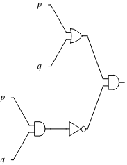
Now we can define a new variable for the output of every gate. For example, we can define $x$ to be the output of the $\textsf{OR}$ gate at the top, $y$ to be the output of the $\textsf{AND}$ gate in the bottom left, and $z$ to be the output of the $\textsf{NOT}$ gate in the bottom right.

Alternatively, you can consider this as defining each subexpression by its own variable; i.e., the above example would lead to the following definitions:

$$ (\overbrace{p\lor q}^x)\land\overbrace{\lnot(\overbrace{p\land q}^y)}^z $$

With these definitions the expression can be written in CNF by $x\land z$ (i.e., the two unit clauses $x$ and $z$) except we also need to represent the definitions of $x$ and $z$ in CNF.

To do this it is conveinient to define a "equivalence" operator $\leftrightarrow$ with the understanding that $x\leftrightarrow y$ means that $x$ and $y$ always take on the same truth value. This operator is sometimes called $\textsf{XNOR}$ because its truth table is the negation of $\textsf{XOR}$:

$$

\begin{array}{cc|ccc} p&q&p&\leftrightarrow&q\\\hline 1&1&1&\mathbf{1}&1\\ 1&0&1&\mathbf{0}&0\\ 0&1&0&\mathbf{0}&1\\ 0&0&0&\mathbf{1}&0 \end{array}

$$

Now the new variables $x$, $y$, and $z$ can be defined using this equivalence operator:

$$ x \leftrightarrow (p\lor q),\qquad y\leftrightarrow(p\land q),\qquad z\leftrightarrow\lnot y $$

Furthermore, it is simple to find equivalent CNF expressions for each of these (e.g., using the first method from above). The following are simple CNF expressions for each:

\begin{gather*} (\lnot x\lor p\lor q)\land(\lnot p\lor x)\land(\lnot q\lor x) \\ (y\lor\lnot p\lor\lnot q)\land(\lnot y\lor p)\land(\lnot y\lor q) \\ (y\lor z)\land(\lnot y\lor\lnot z) \end{gather*}

Putting it all together, the using the Tseitin transformation on the expression $(p\lor q)\land\lnot(p\land q)$ results in the equisatisfiable expression

$$ x\land z\land(\lnot x\lor p\lor q)\land(\lnot p\lor x)\land(\lnot q\lor x)\land(y\lor\lnot p\lor\lnot q)\land(\lnot y\lor p)\land(\lnot y\lor q)\land(y\lor z)\land(\lnot y\lor\lnot z) . $$

Note

It is not always strictly necessary to use a new variable for every subexpression; in this case one could get away with only introducing the variable $u$ defined by $u\leftrightarrow\lnot(p\land q)$ and now the Tseitin transformation would produce the shorter equisatisfiable expression

$$ (p\lor q)\land u\land(\lnot u\lor\lnot p\lor\lnot q)\land(p\lor u)\land(q\lor u) . $$

Cost analysis

We'll now analyze the running time of the Tseitin transformation. Suppose that $n$ is an upper bound on the number of operators in the input expression. For every operator in the expression the Tseitin transformation defines a new variable to represent its output. As seen above, there are at most 3 new clauses which define this variable and each can be generated in constant time.

All operators can be given a variable in linear time by traversing through the circuit. Then the final output variable conjoined with the clauses defining all the new variables can be output as the CNF expression of the input. Thus there will be at most $3n+1$ clauses in the output. In total, generating and outputting these clauses requires $O(n)$ time.

The Davis–Putnam procedure

Now that we've seen how to translate arbitrary Boolean expressions into CNF in linear time we'll assume that all input is given in CNF. This assumption is very useful when designing satisfiability solving algorithms like the Davis–Putnam procedure—originally designed by Martin Davis and Hilary Putnam in 1960.

The fact that the input is in CNF means that a expression is satisfiable exactly when there is an assignment that makes at least one literal in every clause true.

CNF expressions can be represented much easier than arbitrary Boolean expressions (where operators can be nested arbitrarily deeply). Instead of representing an expression by a circuit a CNF expression can be represented by a set of clauses. Also, clauses themselves can be represented by a set of literals.

For example, the expression $(p\lor q)\land u\land(\lnot u\lor\lnot p\lor\lnot q)\land(p\lor u)\land(q\lor u)$ from above could be represented by

$$ \bigl\{ \{p,q \}, \{u\}, \{\lnot u,\lnot p,\lnot q\}, \{p,u\}, \{q,u\} \bigr\} . $$

The resolution rule

The Davis–Putnam procedure is based on the resolution rule which says that if

$$ \{p_1,\dotsc,p_n,r\} \text{ and } \{q_1,\dotsc,q_m,\lnot r\} \text{ hold then } \{ p_1,\dotsc,p_n,q_1,\dotsc,q_m \} \text{ also holds.} $$

In other words, if a variable $r$ appears positively in one clause in negatively in another clause then those clauses can be "merged" together with the variable $r$ removed.

Intuitively the reasoning behind the rule is clear: if $r$ is false then since the first assumed clause holds it must be the case that $\{p_1,\dotsc,p_n\}$ holds and if $r$ is true then $\lnot r$ is false and since the second assumed clause holds it must be the case that $\{q_1,\dotsc,q_m\}$ holds.

In either case a subset of the conclusion holds—implying that the conclusion itself holds.

Example

From $\{\lnot u,\lnot p,\lnot q\}$ and $\{p,u\}$ using the resolution rule on $u$ we derive $\{\lnot p,\lnot q,p\}$. Note that this clause is trivially satisfiable since it includes both $p$ and $\lnot p$.

Description of the procedure

Step 1. If any clause includes $p$ and $\lnot p$ for the same variable $p$ then it is trivally satisfiable and can be removed.

Step 2. If a variable always appears positively in every clause then that variable can simply be assigned to be true and those clauses removed (as they are now satisfied). Conversely, if a variable always appears negatively then that variables can be assigned to be false and the clauses in which it appears can be removed. If after removing clauses there are no more left then you can stop as the entire expression has been satisfied.

Step 3. Choose a variable $p$ that appears positively in at least one clause and negatively in at least one clause. Let $A$ be the set of clauses where $p$ appears and $B$ be the set of clauses where $\lnot p$ appears. Perform resolution on $p$ between all clauses in $A$ and all clauses in $B$ and add the clauses that result into the set of clauses. After this, remove all clauses that include $p$ or $\lnot p$. (This transforms the expression into a equisatisfiable one in which the variable $p$ does not appear.)

Step 4. If the above step introduced the empty clause then stop and output that the formula is unsatisfiable. No assignment satisfies the empty clause—a clause is true when at least one literal in it is true but in a clause that contains no literals this never happens.

Step 5. Continue to repeat the above steps until either the input has been determined to be satisfiable or unsatisfiable.

Example

Let's use the same input from above, i.e., $$ \bigl\{ \{p,q \}, \{u\}, \{\lnot u,\lnot p,\lnot q\}, \{p,u\}, \{q,u\} \bigr\} . $$

Step 1 does not apply; no clauses are trivially satisfiable.

Step 2 does not apply; no variable appears as purely positive or purely negative in the clauses.

In step 3 we need to choose a variable on which to perform resolution; let's use $p$. Then $A:=\{\{p,q\},\{p,u\}\}$ and $B:=\{\{\lnot u,\lnot p,\lnot q\}\}$.

Resolution on $p$ with $\{p,q\}$ and $\{\lnot u,\lnot p,\lnot q\}$ gives $\{q,\lnot u,\lnot q\}$.

Resolution on $p$ with $\{p,u\}$ and $\{\lnot u,\lnot p,\lnot q\}$ gives $\{u, \lnot u, \lnot q\}$.

We now add these clauses to our clause set and remove the clauses with $p$, thereby transforming our input expression to

$$ \bigl\{ \{u\}, \{q,u\}, \{q,\lnot u,\lnot q\}, \{u,\lnot u, \lnot q\} \bigr\} . $$

Step 4 does not apply; the empty clause does not appear.

We return to step 1 and see that the last two clauses are trivially satisfied and can be removed, giving us the clause set

$$ \bigl\{ \{u\}, \{q,u\} \bigr\} . $$

In step 2, now both $u$ only appears positively so by setting $u$ to true we satisfy both clauses and are left with the clause set

$$ \bigl\{ \bigr\} $$

so there are no more clauses to be satisfied and we output satisfiable.

Cost analysis

First, are we even sure that the procedure will necessarily terminate?

Yes, because step 3 removes a variable from the clause set. If the clause set initially has $n$ variables then step 3 can run at most $n$ times. Thus the procedure must terminate as you will go back to step 1 at most $n$ times.

Steps 1, 2, and 4 can all essentially be done in linear time (in the total number of literals appearing in the clause set) as well since they require iterating over every literal in every clause.

So what's the problem? The issue is that step 3 can cause the number of clauses to grow substantially. Say that $p$ appears in half the clauses and $\lnot p$ appears in the other half of the clauses.

If there are $k$ clauses then $|A|$ will be of size $k/2$ and $|B|$ will also be of size $k/2$ and performing resolution on every clause from $A$ and $B$ will result in $(k/2)^2=k^2/4$ new clauses being generated. However, since step 3 will be run up to $n$ times even doubling the size of the clause set would result in an exponential running time in $n$.

Boolean Constraint Propagation

There is one additional improvement to the Davis–Putnam procedure that is extremely useful in practice. Whenever the clause set contains a unit clause then there is only one possible way of satisfying that clause so the value of that variable can be fixed (to true if the unit clause is positive and to false if the unit clause is negative).

For example, the positive unit clause $\{u\}$ appears in the clauses from above $$ \bigl\{ \{p,q \}, \{u\}, \{\lnot u,\lnot p,\lnot q\}, \{p,u\}, \{q,u\} \bigr\} . $$

Thus we can assign $u$ to true and this often allows simplifying many other clauses: any clause that contains $u$ is now automatically satisfied and can be removed. Also, $\lnot u$ can be dropped from any clause that contains it, since $\lnot u$ is now always false. These simplifications are known as Boolean constraint propagation or BCP.

Also note that BCP on a unit clause $\{u\}$ is equivalent to applying the resolution rule to the sets $A:=\{\{u\}\}$ and $B:=\{\,\text{clauses that contain $\lnot u$}\,\}$ (and then removing the clauses containing $u$).

For example, applying BCP to the above clause set gives

$$ \bigl\{ \{p,q \}, \{\lnot p,\lnot q\} \bigr\} . $$

BCP should also be applied repeatedly, since the simplification process may have introduced other unit clauses in the clause set. In fact, modern SAT solvers spend most of their time performing BCP and because of this they use specialized data structures that make performing BCP as fast as possible.

For example, consider the clause set

$$ \bigl\{ \{\lnot p, q\}, \{\lnot q, \lnot r\}, \{r, u\}, \{r, \lnot u \}, \{ p \} \bigr\} . $$

Applying BCP on the unit clause $\{p\}$:

$$ \bigl\{ \{q\}, \{\lnot q, \lnot r\}, \{r, u\}, \{r, \lnot u \} \bigr\} $$

Applying BCP on the unit clause $\{q\}$:

$$ \bigl\{ \{\lnot r\}, \{r, u\}, \{r, \lnot u \} \bigr\} $$

Applying BCP on the unit clause $\{\lnot r\}$:

$$ \bigl\{ \{u\}, \{\lnot u \} \bigr\} $$

Now applying resolution on $u$ on $\{u\}$ and $\{\lnot u \}$ gives the empty clause:

$$ \bigl\{ \{\} \bigr\} $$

This is unsatisfiable, since no assignment satisfies the empty clause.

Important note: Pay particular attention to the difference between $\bigl\{ \bigr\}$ and $\bigl\{ \{\} \bigr\}$! The former is trivially satisfiable (as there are no clauses to satisfy) and the latter is trivially unsatisfiable (because nothing satisfies the empty clause).

The Davis–Putnam–Logemann–Loveland Procedure

In 1962, Davis, Logemann, and Loveland published a second satisfiability solving algorithm that is now known as the "DPLL algorithm" after the initials of Davis and Putnam (since it is based on the Davis–Putnam procedure) as well as Logemann and Loveland.

Apparently the DPLL algorithm was developed when Logemann and Loveland tried to implement the Davis–Putnam procedure on an IBM 704 and found that it used too much memory.

Although the two algorithms are similar, the primary benefit that the DPLL algorithm has over the Davis–Putnam procedure is that the clause set does not increase in size.

Description of the algorithm

Step 1. Repeatedly perform BCP on the set of clauses until no unit clauses exist in the set of clauses $C$.

Step 2. If there are no clauses left in $C$ then return $\textsf{SAT}$.

Step 3. If $C$ contains the empty clause then return $\textsf{UNSAT}$.

Step 4. Choose a variable $p$ that appears in at least one clause to "branch" on.

Recursively call the algorithm on $C\cup\bigl\{\{p\}\bigr\}$ and return $\textsf{SAT}$ if it does so. Otherwise, recursively call the algorithm on $C\cup\bigl\{\{\lnot p\}\bigr\}$ and return that result.

Example

Consider the same set of clauses from above $$ \bigl\{ \{p,q \}, \{u\}, \{\lnot u,\lnot p,\lnot q\}, \{p,u\}, \{q,u\} \bigr\} . $$

In step one we apply BCP on the unit clause $\{u\}$, resulting in $$ \bigl\{ \{p,q \}, \{\lnot p,\lnot q\} \bigr\} . $$

Now BCP does not apply but also clauses remain and they are all nonempty so we move to step 4.

In step 4 we have to branch on either $p$ or $q$; let's say we use $p$. Then we restart the algorithm with the clause set

$$ \bigl\{ \{p,q \}, \{\lnot p,\lnot q\}, \{p\} \bigr\} . $$

Now BCP can be applied on the unit clause $\{p\}$, resulting in

$$ \bigl\{ \{\lnot q\} \bigr\} , $$

from which BCP can be applied on the unit clause $\{\lnot q\}$, resulting in $\bigl\{\bigr\}$ and the algorithm returns $\textsf{SAT}$.

Cost analysis

BCP never increases the size of the clause set: it removes or shrinks clauses. Each time step 1 runs the number of times BCP is applied is bounded by $n$ (the number of variables) since each pass removes one variable.

Steps 2 and 3 clearly can be done in linear time in the size of the clause set.

Step 4 adds a unit clause to the set of clauses but this will actually decrease the number of clauses since BCP will be immediately applied as soon as the recursive call is made.

Then what's the problem here? The issue is that in the worst case the number of recursive calls will be $2^n$ (when every single possible assignment on the $n$ variables is tried separately). One nice way of visualizing this is using a binary tree where each left branch of the tree denotes assigning a variable to true and each right branch denotes assigning a value to false.

The DPLL example from above then produces the following tree:

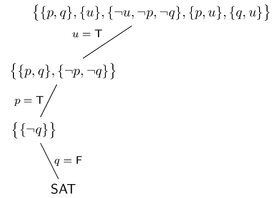
In the above example there is only a single path to the bottom because it just so happened that the first choices for truth values of the variables led to a satisfying assignment. Usually the algorithm won't be so lucky and in general will have to examine all $2^n$ possible assignments, like in this example:

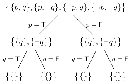
Note that an $\mathsf{UNSAT}$ result at a leaf does not imply the entire expression is unsatisfiable because it's possible that some variables were assigned to be the "wrong" value somewhere along the way.

Reaching a leaf means that one recursive call returns $\mathsf{UNSAT}$ but in general there will be more recursive calls remaining in the algorithm (using different truth assignments). Eventually all recursive calls will complete and if they all return $\mathsf{UNSAT}$ then the entire formula is also $\mathsf{UNSAT}$.

Relationship between DP and DPLL

The DPLL algorithm can be viewed as a variant of the Davis–Putnam procedure where the resolution rule is only applied with unit clauses—this is sometimes called unit resolution.

Furthermore, in DPLL variables are removed by assigning them a fixed value whereas in DP variables are removed by applying repeatedly applying the resolution rule.

The downside of the DP procedure is that the set of clauses can explode in size. The downside of the DPLL algorithm is that when you fix a variable a value and end up with an $\textsf{UNSAT}$ result it might be because you fixed the variable to the "wrong" value. Thus, you have to backtrack and try fixing the variable to the other value.

Conflict-driven Clause Learning

In 1996, Marques-Silva and Sakallah introduced the idea of conflict-driven clause learning (CDCL) and non-chronological backtracking that greatly improved the effectiveness of SAT solvers in practice.

This resulted in what has been called a "SAT revolution" and the usage of SAT solvers to solve a huge variety of problems—even many industrial problems that have nothing to do with logic! For example, today hardware and software verification methods crucially rely on SAT solvers using conflict-driven clause learning.

The CDCL idea

When DPLL reaches a conflict it has to backtrack and try another assignment. However, the CDCL insight is that when a conflict is reached the solver can learn a reason why a conflict occurred. The reason for the conflict can be added as a new clause that must be satisfied going forward.

The learned clause will prevent the solver from reaching the same conflict—but it will also often prevent the solver from reaching many other conflicts in the future because often many branches of the search tree are unsatisfiable for the same underlying reason.

Non-chronological backtracking

Additionally, there is no inherent reason that the search tree in DPLL has to be searched in such an orderly fashion.

For example, suppose after setting $p$, $q$, and $r$ to true a conflict is reached. The DPLL algorithm would now backtrack a level in the tree and keep $p$ and $q$ as set to true but set $r$ to false. Conversely, the CDCL method can jump back several levels; perhaps it keeps $p$ true but then decides to ignore $q$ and $r$ and instead tries setting $u$ to false.

This is known as non-chronological backtracking or backjumping and it gives CDCL more flexibility to explore parts of the search space that are more promising.

It also means that the search tree is no longer binary: at a given node $N$ CDCL might decide to set $p$, then reach a conflict and backjump to $N$ and set $q$, then reach another conflict and backjump to $N$ and set $r$, etc.

How to learn a conflict clause

The simplest thing to learn would be a clause saying that at least one variable value has to be chosen differently. For example, suppose you've set $u=\textsf{T}$, $p=\textsf{T}$, and $q=\textsf{F}$ and then reached a conflict. In this case you could learn the clause $\{\lnot u,\lnot p, q\}$ which says that at least one of your decisions was a mistake.

However, you typically do not want to include the assignments derived by BCP in the conflict clause and only include the decision variables (i.e., the variables whose values were decided on but not derived by BCP).

For example, in the above example if $q$ was assigned because of BCP (i.e., the unit clause $\{\lnot q\}$ was derived after $p$ was set) then you can just learn the conflict clause $\{\lnot u,\lnot p\}$ instead of $\{\lnot u,\lnot p, q\}$.

The reason this works is because all variable assignments from BCP are "forced" from the original clauses and the assignments to the decision variables. Thus if you start from the original clauses and make the same assignments to the decision variables you will still end up with an unsatisfiable expression.

Conflict clauses generated this way only include literals relevant to the conflict and thus produce smaller conflicts. Shorter clauses are stronger, and thus this method is preferable.

The above description of learning a conflict clause only containing the decision variables is the original strategy derived by Marques-Silva and Sakallah. However, it is not the only possible conflict clause and we will see methods of generating conflicts which are better in practice.

Example

Suppose we have the following set of clauses as input:

\begin{align*} c_0 &= \{x_0,x_3\} \\ c_1 &= \{x_0,\lnot x_2,\lnot x_5\} \\ c_2 &= \{x_0,x_5,x_9\} \\ c_3 &= \{x_1,x_8\} \\ c_4 &= \{\lnot x_4,\lnot x_2,x_6\} \\ c_5 &= \{\lnot x_4, x_5, \lnot x_6\} \\ c_6 &= \{x_4,x_5,\lnot x_7\} \\ c_7 &= \{\lnot x_0,x_4,x_7\} \\ c_8 &= \{x_2,x_4,\lnot x_8\} \\ c_9 &= \{\lnot x_1, \lnot x_4\} \end{align*}

For simplicity, we'll always select the unassigned variable with the smallest index as the next decision variable.

In what follows we'll use ${\color{green}{\text{green}}}$ to denote a satisfied literal or clause and ${\color{red}{\text{red}}}$ to denote a literal assigned to false under the current partial assigment.

Thus, $x_0$ is selected as the first decision variable. Say that we set it to false:

\begin{align*} c_0 &= \{{\color{red}{x_0}},x_3\} \\ c_1 &= \{{\color{red}{x_0}},\lnot x_2,\lnot x_5\} \\ c_2 &= \{{\color{red}{x_0}},x_5,x_9\} \\ c_3 &= \{x_1,x_8\} \\ c_4 &= \{\lnot x_4,\lnot x_2,x_6\} \\ c_5 &= \{\lnot x_4, x_5, \lnot x_6\} \\ c_6 &= \{x_4,x_5,\lnot x_7\} \\ \color{green}{c_7} &= \{{\color{green}{\lnot x_0}},x_4,x_7\} \\ c_8 &= \{x_2,x_4,\lnot x_8\} \\ c_9 &= \{\lnot x_1, \lnot x_4\} \end{align*}

Thus first clause $c_0$ is now unit, so $x_3$ must be set to true:

\begin{align*} \color{green}{c_0} &= \{{\color{red}{x_0}},{\color{green}{x_3}}\} \\ c_1 &= \{{\color{red}{x_0}},\lnot x_2,\lnot x_5\} \\ c_2 &= \{{\color{red}{x_0}},x_5,x_9\} \\ c_3 &= \{x_1,x_8\} \\ c_4 &= \{\lnot x_4,\lnot x_2,x_6\} \\ c_5 &= \{\lnot x_4, x_5, \lnot x_6\} \\ c_6 &= \{x_4,x_5,\lnot x_7\} \\ \color{green}{c_7} &= \{{\color{green}{\lnot x_0}},x_4,x_7\} \\ c_8 &= \{x_2,x_4,\lnot x_8\} \\ c_9 &= \{\lnot x_1, \lnot x_4\} \end{align*}

Now $x_1$ is selected as the next decision variable. Say we set it to false:

\begin{align*} \color{green}{c_0} &= \{{\color{red}{x_0}},{\color{green}{x_3}}\} \\ c_1 &= \{{\color{red}{x_0}},\lnot x_2,\lnot x_5\} \\ c_2 &= \{{\color{red}{x_0}},x_5,x_9\} \\ c_3 &= \{{\color{red}{x_1}},x_8\} \\ c_4 &= \{\lnot x_4,\lnot x_2,x_6\} \\ c_5 &= \{\lnot x_4, x_5, \lnot x_6\} \\ c_6 &= \{x_4,x_5,\lnot x_7\} \\ \color{green}{c_7} &= \{{\color{green}{\lnot x_0}},x_4,x_7\} \\ c_8 &= \{x_2,x_4,\lnot x_8\} \\ \color{green}{c_9} &= \{{\color{green}{\lnot x_1}}, \lnot x_4\} \end{align*}

Now $c_3$ is a unit clause, so $x_8$ must be true:

\begin{align*} \color{green}{c_0} &= \{{\color{red}{x_0}},{\color{green}{x_3}}\} \\ c_1 &= \{{\color{red}{x_0}},\lnot x_2,\lnot x_5\} \\ c_2 &= \{{\color{red}{x_0}},x_5,x_9\} \\ \color{green}{c_3} &= \{{\color{red}{x_1}},{\color{green}{x_8}}\} \\ c_4 &= \{\lnot x_4,\lnot x_2,x_6\} \\ c_5 &= \{\lnot x_4, x_5, \lnot x_6\} \\ c_6 &= \{x_4,x_5,\lnot x_7\} \\ \color{green}{c_7} &= \{{\color{green}{\lnot x_0}},x_4,x_7\} \\ c_8 &= \{x_2,x_4,{\color{red}{\lnot x_8}}\} \\ \color{green}{c_9} &= \{{\color{green}{\lnot x_1}}, \lnot x_4\} \end{align*}

No clauses are unit. Now $x_2$ is selected as the next decision variable. Say we set it to true:

\begin{align*} \color{green}{c_0} &= \{{\color{red}{x_0}},{\color{green}{x_3}}\} \\ c_1 &= \{{\color{red}{x_0}},{\color{red}{\lnot x_2}},\lnot x_5\} \\ c_2 &= \{{\color{red}{x_0}},x_5,x_9\} \\ \color{green}{c_3} &= \{{\color{red}{x_1}},{\color{green}{x_8}}\} \\ c_4 &= \{\lnot x_4,{\color{red}{\lnot x_2}},x_6\} \\ c_5 &= \{\lnot x_4, x_5, \lnot x_6\} \\ c_6 &= \{x_4,x_5,\lnot x_7\} \\ \color{green}{c_7} &= \{{\color{green}{\lnot x_0}},x_4,x_7\} \\ \color{green}{c_8} &= \{{\color{green}{x_2}},x_4,{\color{red}{\lnot x_8}}\} \\ \color{green}{c_9} &= \{{\color{green}{\lnot x_1}}, \lnot x_4\} \end{align*}

Now $c_1$ is a unit clause and implies that $x_5$ is false:

\begin{align*} \color{green}{c_0} &= \{{\color{red}{x_0}},{\color{green}{x_3}}\} \\ \color{green}{c_1} &= \{{\color{red}{x_0}},{\color{red}{\lnot x_2}},{\color{green}{\lnot x_5}}\} \\ c_2 &= \{{\color{red}{x_0},\color{red}{x_5}},x_9\} \\ \color{green}{c_3} &= \{{\color{red}{x_1}},{\color{green}{x_8}}\} \\ c_4 &= \{\lnot x_4,{\color{red}{\lnot x_2}},x_6\} \\ c_5 &= \{\lnot x_4, {\color{red}{x_5}}, \lnot x_6\} \\ c_6 &= \{x_4,{\color{red}{x_5}},\lnot x_7\} \\ \color{green}{c_7} &= \{{\color{green}{\lnot x_0}},x_4,x_7\} \\ \color{green}{c_8} &= \{{\color{green}{x_2}},x_4,{\color{red}{\lnot x_8}}\} \\ \color{green}{c_9} &= \{{\color{green}{\lnot x_1}}, \lnot x_4\} \end{align*}

Now $c_2$ is a unit clause and implies that $x_9$ is true:

\begin{align*} \color{green}{c_0} &= \{{\color{red}{x_0}},{\color{green}{x_3}}\} \\ \color{green}{c_1} &= \{{\color{red}{x_0}},{\color{red}{\lnot x_2}},{\color{green}{\lnot x_5}}\} \\ \color{green}{c_2} &= \{{\color{red}{x_0}},{\color{red}{x_5}},{\color{green}{x_9}}\} \\ \color{green}{c_3} &= \{{\color{red}{x_1}},{\color{green}{x_8}}\} \\ c_4 &= \{\lnot x_4,{\color{red}{\lnot x_2}},x_6\} \\ c_5 &= \{\lnot x_4, {\color{red}{x_5}}, \lnot x_6\} \\ c_6 &= \{x_4,{\color{red}{x_5}},\lnot x_7\} \\ \color{green}{c_7} &= \{{\color{green}{\lnot x_0}},x_4,x_7\} \\ \color{green}{c_8} &= \{{\color{green}{x_2}},x_4,{\color{red}{\lnot x_8}}\} \\ \color{green}{c_9} &= \{{\color{green}{\lnot x_1}}, \lnot x_4\} \end{align*}

No clauses are unit. Now $x_4$ is selected as the next decision variable. Say we set it to true:

\begin{align*} \color{green}{c_0} &= \{{\color{red}{x_0}},{\color{green}{x_3}}\} \\ \color{green}{c_1} &= \{{\color{red}{x_0}},{\color{red}{\lnot x_2}},{\color{green}{\lnot x_5}}\} \\ \color{green}{c_2} &= \{{\color{red}{x_0}},{\color{red}{x_5}},{\color{green}{x_9}}\} \\ \color{green}{c_3} &= \{{\color{red}{x_1}},{\color{green}{x_8}}\} \\ c_4 &= \{{\color{red}{\lnot x_4}},{\color{red}{\lnot x_2}},x_6\} \\ c_5 &= \{{\color{red}{\lnot x_4}},{\color{red}{x_5}}, \lnot x_6\} \\ \color{green}{c_6} &= \{{\color{green}{x_4}},{\color{red}{x_5}},\lnot x_7\} \\ \color{green}{c_7} &= \{{\color{green}{\lnot x_0}},{\color{green}{x_4}},x_7\} \\ \color{green}{c_8} &= \{{\color{green}{x_2}},{\color{green}{x_4}},{\color{red}{\lnot x_8}}\} \\ \color{green}{c_9} &= \{{\color{green}{\lnot x_1}}, {\color{red}{\lnot x_4}}\} \end{align*}

Now $c_4$ and $c_5$ are in conflict: to make $c_4$ true we have to assign $x_6$ to true but to make $c_5$ true we would have to assign $x_6$ to false.

Because we made the decisions $x_0=x_1=\textsf{F}$ and $x_2=x_4=\textsf{T}$ the decision literals are $\lnot x_0$, $\lnot x_1$, $x_2$, and $x_4$.

We can form a conflict clause taking the negation of each of the decision literals; call this clause $c_{10}$:

$$c_{10} = \{{\color{red}{x_0}},{\color{red}{x_1}},{\color{red}{\lnot x_2}},{\color{red}{\lnot x_4}}\}.$$

This says that at least one of our decisions has to be changed—which we know must be true since using those decisions we derived a conflict.

We can now add $c_{10}$ into the set of clauses and backtrack. The simplest thing to do would be to undo the last variable assignment $x_4=\textsf{T}$. Then the updated set of clauses would be

\begin{align*} \color{green}{c_0} &= \{{\color{red}{x_0}},{\color{green}{x_3}}\} \\ \color{green}{c_1} &= \{{\color{red}{x_0}},{\color{red}{\lnot x_2}},{\color{green}{\lnot x_5}}\} \\ \color{green}{c_2} &= \{{\color{red}{x_0}},{\color{red}{x_5}},{\color{green}{x_9}}\} \\ \color{green}{c_3} &= \{{\color{red}{x_1}},{\color{green}{x_8}}\} \\ c_4 &= \{{{\lnot x_4}},{\color{red}{\lnot x_2}},x_6\} \\ c_5 &= \{{{\lnot x_4}},{\color{red}{x_5}}, \lnot x_6\} \\ {c_6} &= \{{{x_4}},{\color{red}{x_5}},\lnot x_7\} \\ \color{green}{c_7} &= \{{\color{green}{\lnot x_0}},{{x_4}},x_7\} \\ \color{green}{c_8} &= \{{\color{green}{x_2}},{{x_4}},{\color{red}{\lnot x_8}}\} \\ \color{green}{c_9} &= \{{\color{green}{\lnot x_1}}, {{\lnot x_4}}\} \\ c_{10} &= \{{\color{red}{x_0}},{\color{red}{x_1}},{\color{red}{\lnot x_2}},{{\lnot x_4}}\} \end{align*}

Now $c_{10}$ is a unit clause and implies that $x_4$ must be set to false:

\begin{align*} \color{green}{c_0} &= \{{\color{red}{x_0}},{\color{green}{x_3}}\} \\ \color{green}{c_1} &= \{{\color{red}{x_0}},{\color{red}{\lnot x_2}},{\color{green}{\lnot x_5}}\} \\ \color{green}{c_2} &= \{{\color{red}{x_0}},{\color{red}{x_5}},{\color{green}{x_9}}\} \\ \color{green}{c_3} &= \{{\color{red}{x_1}},{\color{green}{x_8}}\} \\ \color{green}{c_4} &= \{{\color{green}{\lnot x_4}},{\color{red}{\lnot x_2}},x_6\} \\ \color{green}{c_5} &= \{{\color{green}{\lnot x_4}},{\color{red}{x_5}}, \lnot x_6\} \\ {c_6} &= \{{\color{red}{x_4}},{\color{red}{x_5}},\lnot x_7\} \\ \color{green}{c_7} &= \{{\color{green}{\lnot x_0}},{\color{red}{x_4}},x_7\} \\ \color{green}{c_8} &= \{{\color{green}{x_2}},{\color{red}{x_4}},{\color{red}{\lnot x_8}}\} \\ \color{green}{c_9} &= \{{\color{green}{\lnot x_1}}, {\color{green}{\lnot x_4}}\} \\ \color{green}{c_{10}} &= \{{\color{red}{x_0}},{\color{red}{x_1}},{\color{red}{\lnot x_2}},{\color{green}{\lnot x_4}}\} \end{align*}

Now $c_6$ is a unit clause and implies that $x_7$ must be set to false:

\begin{align*} \color{green}{c_0} &= \{{\color{red}{x_0}},{\color{green}{x_3}}\} \\ \color{green}{c_1} &= \{{\color{red}{x_0}},{\color{red}{\lnot x_2}},{\color{green}{\lnot x_5}}\} \\ \color{green}{c_2} &= \{{\color{red}{x_0}},{\color{red}{x_5}},{\color{green}{x_9}}\} \\ \color{green}{c_3} &= \{{\color{red}{x_1}},{\color{green}{x_8}}\} \\ \color{green}{c_4} &= \{{\color{green}{\lnot x_4}},{\color{red}{\lnot x_2}},x_6\} \\ \color{green}{c_5} &= \{{\color{green}{\lnot x_4}},{\color{red}{x_5}}, \lnot x_6\} \\ \color{green}{c_6} &= \{{\color{red}{x_4}},{\color{red}{x_5}},\color{green}{\lnot x_7}\} \\ \color{green}{c_7} &= \{{\color{green}{\lnot x_0}},{\color{red}{x_4}},\color{red}{x_7}\} \\ \color{green}{c_8} &= \{{\color{green}{x_2}},{\color{red}{x_4}},{\color{red}{\lnot x_8}}\} \\ \color{green}{c_9} &= \{{\color{green}{\lnot x_1}}, {\color{green}{\lnot x_4}}\} \\ \color{green}{c_{10}} &= \{{\color{red}{x_0}},{\color{red}{x_1}},{\color{red}{\lnot x_2}},{\color{green}{\lnot x_4}}\} \end{align*}

Finally we've found an assignment that satisifes all the clauses! The only variable that hasn't been assigned a value is $x_6$, but a value can be given to $x_6$ arbitrarily because the clauses which contain $x_6$ are already satisfied.

Implication graph

The series of propagations made by BCP can be represented by a graph known as the implication graph.

The implication graph is a directed acyclic graph which has a node for every variable assignment made. The root nodes (those without any incoming edges) represent decision variables and every time a variable is set using BCP there are edges to the node representing the variable being set from all the nodes representing the assignments which were involved in making the relevant clause a unit clause.

Additionally, the edges are labelled with the relevant clause used to perform BCP and nodes are labelled with $p$ or $\lnot p$ (corresponding to if $p$ was set to true or false). Nodes also are labelled with a decision level: the current number of decisions made when the variable in that node was assigned.

When a conflict is reached it can also be given a node (with edges from the assignments causing the conflict).

For example, this is the implication graph of the above example once the conflict was reached:

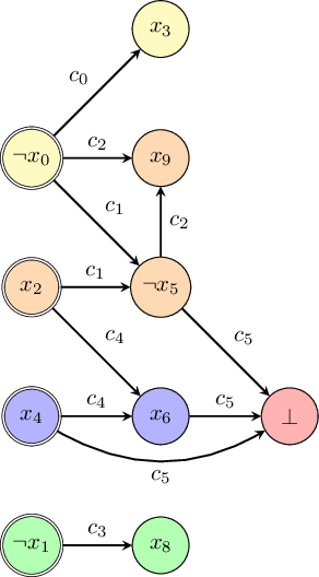
Here the yellow nodes are at decision level 1, the green nodes are at decision level 2, the orange nodes are at decision level 3, the blue nodes are at decision level 4, and the red node denotes the conflict node. The decision nodes are on the left and drawn with a double outline.

Improved conflict clause generation

The purpose of the implication graph is that it facilitates generating better conflict clauses than the method of generating a conflict clause by negating all of the decision literals.

In fact, there are many possible conflict clauses that can be generated from the implication graph. The general method of finding them is to instantiate a set $C$ containing the negations of all parents of the conflict node and then replace one of the entries of $C$ with the negations of all of the parents of that entry.

In the example above, we start with

$$C:=\{\lnot x_4,x_5,\lnot x_6\}$$

(which is $c_5$, the clause that caused the conflict). The parents of $x_6$ are $x_2$ and $x_4$, so we could update $C$ to be

$$(\{\lnot x_4,x_5,\lnot x_6\}\setminus\{\lnot x_6\})\cup\{\lnot x_2,\lnot x_4\} = \{\lnot x_2,\lnot x_4,x_5\} . $$

In fact, this is equivalent to applying the resolution rule on $c_5$ and $c_4$ (the clause used to derive $x_6$).

The parents of $\lnot x_5$ are $x_2$ and $\lnot x_0$, so we could still go one step further and update $C$ to be

$$ (\{\lnot x_2,\lnot x_4,x_5\} \setminus\{ x_5 \})\cup \{x_0,\lnot x_2\} = \{x_0,\lnot x_2,\lnot x_4\} . $$

This is the same conflict clause produced by the first method. Now $C$ cannot be further updated since it consists of the negations of the decision literals (which have no parents).

Unique implication point method

We saw how to generate many different conflict clauses by working backwards through the implication graph, but how do we know which is the best to use? There is no easy answer to this question, but a method that works well in practice is called the unique implication point method.

The idea is that you stop moving backwards in the implication graph as soon as (1) the conflict clause $C$ has only a single node at the current decision level and (2) that node is a unique implication point or "UIP".

A node in the graph is a UIP if every path from the last decision literal to the conflict node passes through it.

For example, consider the partial implication graph below. As before, the yellow nodes have decision level 1, the green node has decision level 2, and the orange nodes have decision level 3.

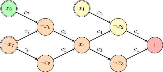
There are four paths between the current decision literal $\lnot x_7$ and the conflict node. They all pass through $\lnot x_7$ and $x_4$, so those both UIPs. However, no other nodes are UIPs since any other node can be avoided in a path from $\lnot x_7$ to $\bot$. For example, you can avoid $\lnot x_2$ by taking the path $\lnot x_7,\lnot x_5,x_4,\lnot x_3,\bot$ and hence $\lnot x_2$ is not a UIP.

Example

We now demonstrate using the UIP method to derive a conflict clause. Recall that in the UIP method we keep updating the conflict clause $C$ until the only node at the current decision level is a UIP.

In the above graph we start with the negations of the parents of the conflict node:

$$ C = \{x_2,x_3\} $$

Now replace $x_3$ (the last assigned literal in $C$) with the negations of the parents of $\lnot x_3$:

$$ C = \{x_2,\lnot x_4\} $$

Now we can stop, since $x_2$ has decision level 1 and $x_4$ is a UIP and has decision level 3.

Conflict clauses via resolution

The generated conflict clauses can be justified by continually applying the resolution rule.

Also note that the set of clauses (at least those involved in the conflict derivation) can be inferred by the implication graph: an edge labelled $c$ in the implication graph which goes from $x$ to $y$ implies that $y$ appears in $c$ and the negation of $x$ appears in $c$. This is because this edge represents applying BCP to clause $c$—so $c$ must be the unit clause $\{y\}$ under the assignment formed by the literals pointing to node $y$.

Using this rule we find that this implication graph was generated using the following clauses:

\begin{align*} \color{red}{c_1} &= \{{\color{red}{x_2}},{\color{red}{x_3}}\} \\ \color{green}{c_2} &= \{{\color{red}{\lnot x_1}},{\color{green}{\lnot x_2}}\} \\ \color{green}{c_3} &= \{{\color{green}{\lnot x_3}},{\color{red}{\lnot x_4}}\} \\ \color{green}{c_4} &= \{{\color{green}{\lnot x_2}},{\color{red}{\lnot x_4}}\} \\ \color{green}{c_5} &= \{{\color{green}{x_4}},{\color{red}{x_5}},{\color{red}{x_6}}\} \\ \color{green}{c_6} &= \{{\color{green}{\lnot x_5}},{\color{red}{x_7}}\} \\ \color{green}{c_7} &= \{{\color{green}{\lnot x_6}},{\color{red}{x_7}},{\color{red}{\lnot x_8}}\} \end{align*}

The decision literals are $x_1$, $\lnot x_7$, and $x_8$, so Marques-Silva and Sakallah's method of conflict clause generation would now learn $\{\lnot x_1,x_7,\lnot x_8\}$.

The UIP method starts with $C:=\{x_2,x_3\}$ (which is just $c_1$) and then updates $C$ to be $\{x_2,\lnot x_4\}$ by applying the resolution rule (on $x_3$) using the clauses $C$ and $c_3$ (the label on the edge pointing to $\lnot x_3$).

How far to backjump?

One last thing: How far should we backtrack once a conflict clause has been generated? In other words, how many variable decisions should we undo? We know we have to undo at least one decision to avoid a conflict but only undoing a single decision is suboptimal in practice.

The method that is used is practice is to backtrack as far as possible as long as the conflict clause is asserting meaning that it can immediately be used to perform BCP (i.e., that it is a unit clause under the current partial assignment).

In other words, we stop backtracking as soon as going any farther would introduce more than one unassigned literal into the conflict clause.

In the example above, the conflict clause generated by the UIP method is $\{x_2,\lnot x_4\}$. Note that $x_2$ has decision level $1$ and $\lnot x_4$ has decision level 3. We can backtrack to decision level 1 while still keeping $C$ asserting; in other words, we can forget the choices made at decision levels 2 and 3.

In general, if the literal $l$ has the second-highest decision level in $C$ then we want to backjump to the decision level of $l$ to keep $C$ asserting. Backjumping any farther would unassign a value to $l$ and therefore require another assignment before BCP could be performed on $C$.

Continuing with the example from above, the conflict clause $C$ is added as a new clause $c_8$ and after the backjump the updated set of clauses would now be:

\begin{align*} {c_1} &= \{{\color{red}{x_2}},{{x_3}}\} \\ \color{green}{c_2} &= \{{\color{red}{\lnot x_1}},{\color{green}{\lnot x_2}}\} \\ {c_3} &= \{{{\lnot x_3}},{{\lnot x_4}}\} \\ \color{green}{c_4} &= \{{\color{green}{\lnot x_2}},{{\lnot x_4}}\} \\ {c_5} &= \{{{x_4}},{{x_5}},{{x_6}}\} \\ {c_6} &= \{{{\lnot x_5}},{{x_7}}\} \\ {c_7} &= \{{{\lnot x_6}},{{x_7}},{{\lnot x_8}}\} \\ c_8 &= \{{\color{red}{x_2}},\lnot x_4\} \end{align*}

And $c_8$ is still asserting and immediately implies that $x_4$ must be set to false. (Technically $c_1$ is also asserting at decision level 1, so this example assumes BCP was not applied on $c_1$ when it could have been.)

Takeaway

The CDCL algorithm described will take exponential time in the worst case since it essentially might have to try every possible assignment before concluding that an expression is unsatisfiable.

In fact, in 1985, Haken showed that there are expressions that are trivially unsatisfiable that CDCL solvers will use exponential time to solve! (At least so long as the internal reasoning of the solver is based on applying the resolution rule.)

Despite this extremely pessimistic result the CDCL algorithm described here actually performs surprisingly well on many cases of interest.

Of course, there are a number of additional strategies that make modern SAT solvers perform well in practice. For example, one important aspect that can have a dramatic effect on the solver's running time is how to decide which variable to branch on. Modern solvers apply various heuristics to select the "most promising" next variable to assign a value to (and to select what value it should be assigned to).

In summary, there is still a lot that we don't know about the SAT problem. We don't know if an efficient algorithm for SAT exists, we don't know if SAT can be solved in polynomial time, and we don't know why the CDCL algorithm and the methods used for generating conflict clauses work well in many cases of interest.

Until we have a more complete understanding of SAT we can at least use the solvers that have been developed—and sometimes solve problems that we don't really have any business solving.

For information on how to solve various mathematical problems with a SAT solver see [1].

References

[1] Bright, Gerhard, Kotsireas, Ganesh. Effective Problem Solving using SAT Solvers. Maple in Mathematics Education and Research, 2020.