Basic Algebraic Operations
This worksheet provides an introduction to representations of basic mathematical objects and how arithmetic can be performed on them.
The fundamental objects we'll consider are integers and polynomials.
The fundamental arithmetic operations we'll consider are addition/subtraction, multiplication, and division.
The “Integer” Datatype
Programming languages such as C allow declaring "int" datatypes.
But "int" is not actually a general integer type. On machines where "int"s are represented by 4 bytes (32-bit) they can only represent integers in the range $-2{,}147{,}483{,}648$ to $2{,}147{,}483{,}647$. On 64-bit machines ints can only represent integers up to around $\pm9.2$ quintillion.
Just as in mathematics, we would like our computations to have no such limitation.
123^45
But wait a minute: the CPU in the computer that we're running on is limited to performing computations on integers of a specific "word size" (typically 64 bits, i.e., 8 bytes).
So how is it possible to perform computations on integers of arbitrary size?
Representation of Integers
The main idea is to split an integer of arbitrary size into "word size" chunks. The base-$2^{64}$ representation of an integer (assuming a word size of size 64 bits) is an appropriate way to achieve this.
Any integer $a$ can be written in the form
$$ a = (-1)^s \sum_i a_i \, 2^{64 i} \notag $$
where $a_i$ are the "base-$2^{64}$ digits" of $a$ (so that $0 \leq a_i < 2^{64}$) and $s$ is 0 or 1, depending on if $a$ is positive or negative.
In other words, arbitrary integers can be represented by a list $[s, a_0, a_1, \dotsc, a_{n-1}]$. Here $n$ is the "length" of an integer and is given by $\lfloor\log_{2^{64}}(a)\rfloor+1$. This expression is a bit unwiedly—to make our lives easier we often analyze things "asymptotically". In this case, it is sufficient to know that $a$ is represented by a list of length $O(\log(a))$.
Example
Let's see an example of this representation:
a = 123^45; print(a)
A = a.digits(base=2^64); print(A)
b = add(A[i]*2^(64*i) for i in range(len(A))); print(b)
print(a==b)
Representation of Polynomials
Polynomials have similar properties to integers in many (but not all) aspects.
A polynomial in the variable $x$ is of the form $f_0 + f_1 x + \dotsb + f_n x^n$ where the $f_i$ are the coefficients of the polynomial and $n$ is the degree of the polynomial (the final coefficient $f_n$ is assumed to not be zero).
If the coefficients are from $\mathbb Z$ (integers) then we write $f\in\mathbb Z[x]$. Other possible domains for the coefficients include $\mathbb Q$ (rational numbers), $\mathbb R$ (real numbers), or $\mathbb C$ (complex numbers). More generally, any algebraic structure that supports addition and multiplication can be used (such structures are called rings).
f = 1 + 2*x + 3*x^2
print(f)
A polynomial can be represented as a list of its coefficients $[f_0, f_1, \dotsc, f_n]$.
f.list()
This is not the only possible representation, but it suffices for now.
Specifying the coefficient ring in Sage
The polynomial $f=1+2x+3x^2$ defined above is an expression in terms of $x$. By default Sage treats x as a symbolic variable in what Sage calls the symbolic ring.
Sage also allows you to control the ring of coefficients to use when constructing and performing operations on polynomials. The following line enables defining polynomials in $x$ over the integers:
R.<x> = ZZ['x']
This line actually defines two things:
- The Sage variable
Rto be $\mathbb Z[x]$ (the ring of polynomials in $x$) - The Sage variable
xto be the symbolic variable'x', the indeterminant ofR
The above definition can also be replaced with R.<x> = ZZ[] because if an explicit symbolic variable is not given Sage will match the indeterminant symbolic variable with the name given to the indeterminant. The syntax R.<x> = PolynomialRing(ZZ) also works.
Note that for some operations the underlying polynomial ring will be important. For example, when $x$ is the indeterminant of $R=\mathbb{Z}[x]$ the polynomial $x^2+1$ does not factor—but if $R=\mathbb{C}[x]$ then the polynomial $x^2+1$ does factor as $(x-i)(x+i)$.
After defining the polynomial ring as above, R can be used as a function which creates polynomials in the ring with a given list of coefficients:
R([1,2,3])
Addition of Polynomials
Addition is one of the simplest arithmetic operations that can be performed on polynomials.
Suppose $f = \sum_{i=0}^n f_i \, x^i$ and $g = \sum_{i=0}^n g_i \, x^i$ and let $h = f + g$ be their sum. We have $h = \sum_{i=0}^n (f_i + g_i) \, x^i$.
In other words, we can add their coefficients pointwise. This leads to a simple algorithm for addition:
for i from 0 to n do
    h[i] = f[i] + g[i]
This uses $n+1 = O(n)$ coefficient additions.
Addition of Integers
This is similar to the polynomial case but already we'll see that the integer arithmetic case is a bit more difficult. For simplicity, we'll assume the numbers are positive and of the same length.
Suppose that $a = \sum_{i=0}^n a_i \, 2^{64 i}$ and $b = \sum_{i=0}^n b_i \, 2^{64 i}$ and let $c = a + b$ be their sum. We have that $c = \sum_{i=0}^n (a_i + b_i) \, 2^{64 i}$.
Is this a valid final answer?
The summation is correct, but it may be the case that $a_i + b_i \geq 2^{64}$ and therefore that $a_i+b_i$ would not be a valid base-$2^{64}$ digit.
Addition of Integers II
First, we can represent $a_0 + b_0 = c_0 + \gamma_0\cdot2^{64}$ where $0\leq c_0<2^{64}$ and $\gamma_0$ is either $0$ or $1$.
Second, we can represent $a_1+b_1+\gamma_0 = c_1 + \gamma_1\cdot2^{64}$ where $0\leq c<2^{64}$ and $\gamma_1$ is either $0$ or $1$. This also works for each remaining coefficient.
This results in the following addition algorithm:
gamma[-1] = 0
for i from 0 to n+1 do
    gamma[i] = 0
    c[i] = a[i] + b[i] + gamma[i-1]
    if c[i] >= 2^64 then
        gamma[i] = 1
        c[i] = c[i] - 2^64
What is the asymptotic complexity in word size additions?
This uses $O(n)$ word size additions. There are $O(n)$ loop iterations and a constant number of additions on each iteration.
The Relationship Between Integers and Polynomials
Note the similarity between the representation $a = \sum_{i=0}^n a_i \, 2^{64 i}$ for (positive) integers and $f = \sum_{i=0}^n f_i x^i$ for polynomials.
Even though integers are perhaps more "familiar" we tend to prioritize the polynomial case in this course—this makes life easier!
Often algorithms that operate on polynomials can be adapted (with a bit of massaging) to work with integers. Not always, however: some algorithms only work on polynomials.
Multiplication of Polynomials
Suppose $f = \sum_{i=0}^n f_i \, x^i$ and $g = \sum_{i=0}^m g_i \, x^i$ and let $h = f \cdot g$ be their product. Then $h = \sum_{i=0}^n (f_i\cdot g) x^i$ and this implies that the product can be found by multiplying $g$ by the coefficients of $f$ and then summing the results together.
This is similar to the integer multiplication algorithm you may have learned in elementary school.
for i from 0 to n do
    h[i] = f[i]*g*x^i
h = add(h[i] for i in range(n))
Example
f = 1 + 2*x + 3*x^2
F = f.list()
g = 4 + 5*x + 6*x^2

print(f.list())
print(g.list())
p = [0, 0, 0]
for i in range(3):
    p[i] = expand(F[i]*g*x^i)
    print(p[i].list())
h = add(p[i] for i in [0..2]); print(h)
print(h==f*g)
Cost in coefficient multiplications and additions
First, line 2 is run $n+1$ times.
Line 2 requires $m+1$ multiplications each time it runs. Note that the multiplication by $x^i$ does not require any coefficient multiplications. Instead, multiplying $f_i\cdot g$ by $x^i$ adds $i$ zeros to the front of its list of coefficients, i.e.,
$$ [f_i\cdot g_0, f_i\cdot g_1, \dotsc, f_i\cdot g_m] \cdot x^i = [\underbrace{0,0,\dotsc,0}_{\text{$i$ zeros}},f_i\cdot g_0, f_i\cdot g_1, \dotsc, f_i\cdot g_m] . $$
Thus, line 2 requires $(n+1)\cdot(m+1)=O(n\cdot m)$ coefficient multiplications.
Line 3 adds together $n+1$ polynomials of maximum degree $n+m$. Thus, this uses $O(n(n+m))$ cofficient additions.
If you are careful and only add together coefficients of the polynomials that are nonzero this actually requires exactly $n\cdot m$ coefficient additions (assuming all $n+1$ coefficients of $f$ and all $m+1$ coefficients of $g$ are nonzero).
Multiplication of integers
A similar algorithm works for multiplication of integers.
It requires $O(n\cdot m)$ word size additions and multiplications in order to multiply an integer of length $n$ with an integer of length $m$.
Division of Polynomials
Given two polynomials $a$ and $b$ the division with remainder problem is to find $q$ and $r$ (quotient and remainder) which satisfy
$$ a = q\cdot b + r \quad\, \text{where} \quad\, \deg(r) < \deg(b) . \notag $$
Caveat: For such a representation to exist the leading coefficient of $b$ must be invertible. Over $\mathbb Z$ this means the leading coefficient must be $\pm1$. Over $\mathbb Q$ or $\mathbb R$ any nonzero coefficient works.
Example
Suppose $b=x^2+2x+3$ and $a=4x^4+5x^3+6x^2+7x+8$.
By hand and some algebraic manipulation you can work out an expression $a=q\cdot b+r$:
\begin{align*} a &= 0\cdot b + 4x^4 + 5x^3 + 6x^2 + 7x + 8 \\ &= (4x^2)\cdot b - 3x^3 - 6x^2 + 7x + 8 \\ &= (4x^2-3x)\cdot b + 16 x + 8 \end{align*}
So $q=4x^2-3x$ and $r=16 x + 8$.
Sage provides a quo_rem function to compute a quotient and remainder simultaneously.
a = 4*x^4 + 5*x^3 + 6*x^2 + 7*x + 8
b = x^2 + 2*x + 3
q, r = a.quo_rem(b)
print([q,r])
Algorithm
Suppose $a$ has degree $n$, $b$ has degree $m$, and the leading coefficient of $b$ is 1 (for simplicity).
r = a
for i from n-m, n-m-1, ..., 0 do
    if deg(r) = m+i then
        q[i] = leading coefficient of r
        # Set the leading coefficient of r to zero
        r = r - q[i]*x^i*b
    else
        q[i] = 0
q = add(q[i]*x^i for i in range(n-m+1))
Sage implementation for polynomial division
# Return the quotient and remainder of a divided by b in R = Z[x]
def division(a, b):
    r = a
    n = a.degree(a)
    m = b.degree(b)
    q = [0 for i in [0..n-m]]
    for i in range(n-m,-1,-1):
        if r.degree() == m+i:
            q[i] = r.leading_coefficient()
            r = r - q[i]*x^i*b
    return R([q[i] for i in [0..n-m]]), r
q, r = division(a, b)
print([q, r])
print(a==q*b+r)
Analysis in coefficient multiplications and additions
The line that updates $r$ requires $O(m)$ multiplications and additions each time it is run, which is at most $n-m+1$ times.
These are the only coefficient additions and multiplications! In total the algorithm uses $O((n-m+1)\cdot m)$ coefficient operations.
Integer case
The same basic algorithm for division works in the integer case but the details are somewhat more complicated.
It uses $O((n-m+1)\cdot m)$ word operations to divide an integer of length $n$ by an integer of length $m$.
Take-aways
Arbitrary-precision integers and polynomials have many similarities.
| Polynomials | Integers | |
|---|---|---|
| size | degree | length |
| algorithm cost | coefficient operations | word operations |
If $a$ and $b$ are polynomials/integers of degree/length $n$ and $m$ then the cost of each algebraic operation is:
- Addition/subtraction: $O(n + m)$
- Multiplication: $O(n\cdot m)$
- Division with remainder: $O((n - m + 1)\cdot m)$
Generally, this means that addition/subtraction run in linear time in the size of the input while multiplication/division run in quadratic time in the size of the input.
An important and interesting problem is now raised: Can we do better?
In the case of addition/subtraction: the classical algorithms are already optimal.
In the case of multiplication/division: yes, we can do better!
Seeing how to solve these and related problems quickly is a driving motivation of this course.
A huge amount of work has gone into solving these problems quicker, both theoretically and in practice.
For example, the GMP library is a C library for arbitrary precision integer arithmetic used by numerous applications such as public-key cryptography and compilers for various programming languages. They have run extensive benchmarks of various algorithms for multiplication:
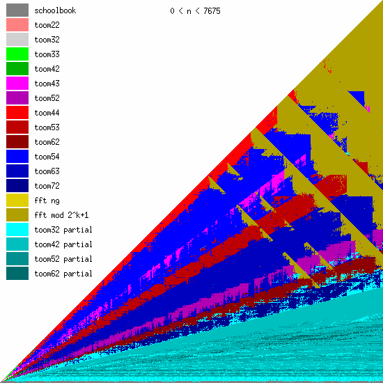
The horizontal axis represents the length of the first operand and the vertical axis represents the length of the second operand (both on a log scale). The colours denote the algorithm that gives the best performance in each case.